In this chapter, we will learn how to predict categories using the logistic regression model.
In logistic regression (classification), the output variable y can take on only one of a small handful of possible values instead of any number in an infinite range of numbers.
Therefore, it turns out that Linear Regression is not a good algorithm for classification problems.
Classification Problem
| Question | Answer “y” |
|---|---|
| Is this email spam? | no or yes |
| Is this transaction fraudulent? | no or yes |
| Is the tumor malignant? | no or yes |
This type of classification problem where there are only two possible outputs is called binary classification.
Where the word binary refers to there being only two possible classes or two possible categories.
In these problems, the terms class and category are used relatively interchangeably.
Binary Classification
y (target output) can only be one of two values.
“Binary” Classification
Example:
no or yes
false or true
0 or 1
NOTE:
In computing convention, 0 refers to false, and 1 refers to true.
Use the numbers zero “0” and one “1” to represent the answer y (target output).
Because that will fit in most easily with the types of learning algorithms we want to implement.
0 is “negative class” (not “bad”) - more like “absence”
1 is “positive class” (not “good”) - more like “presence”
It’s based on the question, for example: is the email spam?
0 means No, it’s not spam
1 means Yes, it’s spam
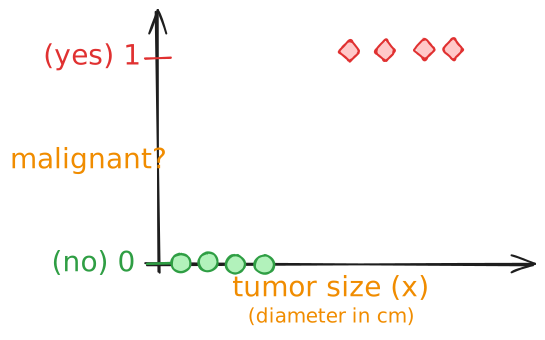
Example of classifying if a tumor is malignant
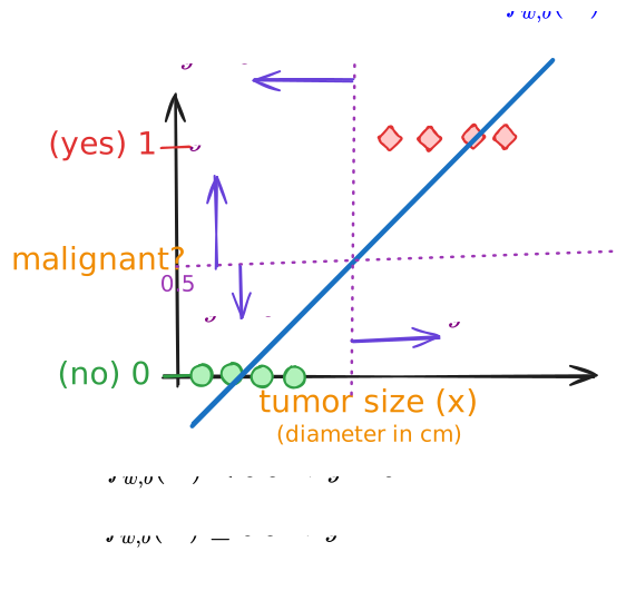
Here’s an example of a training set for classifying if the tumor is malignant.
Classification with Linear Regression!
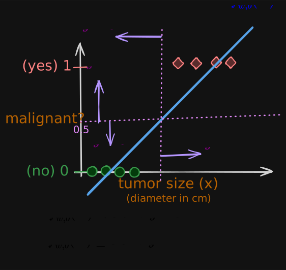
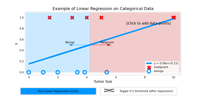
For this example of a training set for classifying if the tumor is malignant, one thing you could try on this training set is to apply the algorithm you already know.
Linear regression and try to fit a straight line to the data.
If you do that, maybe the straight line looks like this, right?
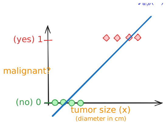
Linear regression predicts not just the values zero and one.
But all numbers between zero and one or even less than zero or greater than one.
But here we want to predict categories.
One thing you could try is to pick a threshold of say 0.5.
So that if the model outputs a value below 0.5, then you predict y equals zero or not malignant. And if the model outputs a number equal to or greater than 0.5, then predict y equals one or malignant.
Notice that this threshold value of 0.5 intersects the best fit straight line at this point. So if you draw this vertical line here, everything to the left ends up with a prediction of y equals zero. And everything on the right ends up with the prediction of y equals one.
Let’s see what happens if your dataset has one more training example.
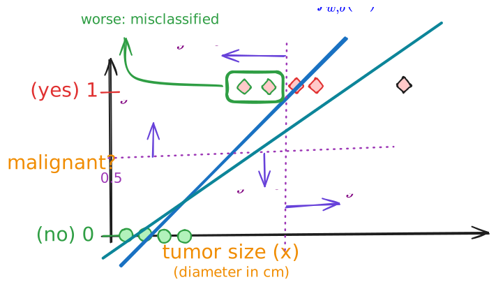
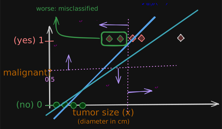
Clearly, when the tumor is large, we want the algorithm to classify it as malignant. So what we just saw was linear regression causes the best fit line.
Adding one more example on the right caused linear regression’s best-fit line to shift, and with it the dividing line, also called the decision boundary, shifted to the right.
It’s better to use “Logistic Regression” where the output will always be between zero and one, and that will avoid these problems.
Another Example:
Logistic Regression
By the way, one confusing thing about the name logistic regression is that even though it has the word regression in it, it is actually used for classification.
It’s actually used to solve binary classification problems where the output label y is either zero or one.
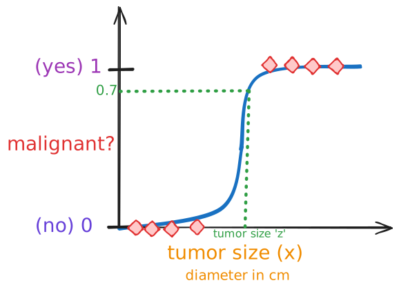
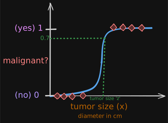
To classify whether a tumor is malignant, fit an S-shaped curve like this to the dataset.
For this example, if a patient comes in with a tumor of size ‘z’, on the x-axis, then the algorithm will output 0.7, suggesting it is more likely to be malignant than benign.
But the output label y is never 0.7.
IT’S ONLY EVER 0 or 1.
To build the logistic regression algorithm, there’s an important mathematical function I’d like to describe, called the sigmoid function, sometimes also referred to as the logistic function.
Sigmoid Function (Logistic Function)
The Sigmoid function looks like this. Notice that the x-axes of the graphs on the left and right are different. In the graph on the left, the x-axis is the tumor size, so it’s all positive numbers.
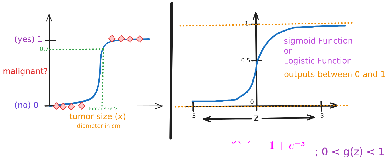
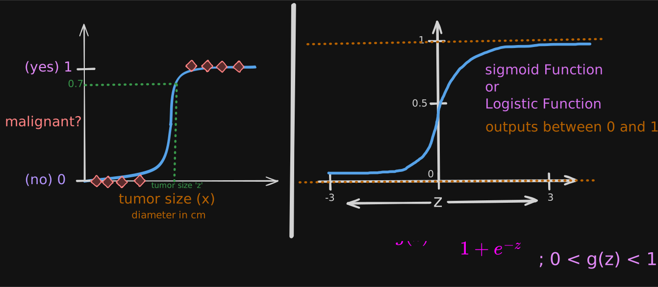
if z = 100, then g(z) will be close to 1.
if z = -100, then g(z) will be close to 0.
if z = 0, then g(z) will be 0.5. (so that’s why it crosses the vertical axis at 0.5)
That’s why the sigmoid function has this shape where it starts very close to zero and slowly builds up or grows to the value of one.
Let’s build: Logistic Regression
We’re going to do this in two steps.
In the first step, I hope you remember that a straight line function, like a linear regression function can be defined as
Let’s store this value in a variable which I’m going to call z,
The next step then is to take this value of z and pass it to the Sigmoid function, also called the logistic function, g.
When you take these two equations and put them together, they then give you the logistic regression model
This is the logistic regression model, and what it does is it inputs a feature or set of features X and outputs a number between 0 and 1.
Interpretation of Logistic Regression Output
One way to think of logistic regression’s output is as the probability that the class or the label y will be equal to 1 given a certain input x.
“probability” that class is 1.
Example
x is “tumor size” y is 0 (not malignant) or 1 (malignant)
what this means is that the model is predicting or the model thinks there’s a 70 percent chance that the true label y would be equal to 1 for this patient.
In other words, the model is telling us that it thinks the patient has a 70 percent chance of the tumor turning out to be malignant.
We know that y has to be either 0 or 1, so if y has a 70 percent chance of being 1, what is the chance that it is 0?
So y has got to be either 0 or 1, and thusthe probabilities of it being 0 or 1 have to add up to one, or 100 percent.
That’s why if the chance of y being 1 is 0.7 or 70 percent chance, then the chance of it being 0 has got to be 0.3 or 30 percent chance.
Adds to 1
In general,
Logistic Notation
What the semicolon here is used to denote is just that w and b are parameters that affect this computation of what is the probability of y being equal to 1 given the input feature x
Real world usage
For a long time, a lot of Internet advertising was actually driven by basically a slight variation of logistic regression. This was very lucrative for some large companies, and this is basically the algorithm that decided what ad was shown to you and many others on some large websites.
Decision Boundary
let’s take a look at the decision boundary to get a better sense of how logistic regression is computing these predictions.
Recap & Intuition
To recap,
where,
This is going to be a number like maybe a 0.7 or 0.3, etc...
what if you want the algorithm to predict whether y is going to be zero or one?
We can set a Threshold above which you predict
Below which
So,
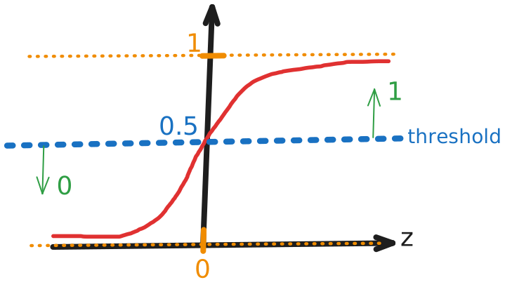
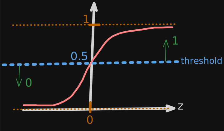
If ?
Yes:
No:
When is 
We recall,
so,
when
when ? Based on above sigmoid graph, when
When is ? Well , so whenever
whenever ,
whenever ,
what about ? well, that depends on the problem we are solving!!!
Visualize how the model makes predictions
Problem 1 - Linear Decision Boundary
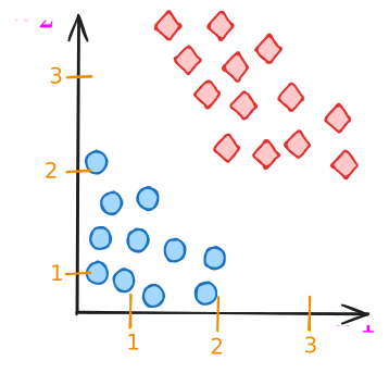
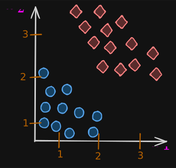
take an example of a classification problem where you have two features, and instead of just one feature. Here’s a training set where the little red diamonds denote the positive examples and the little blue circles denote negative examples.
The red diamonds correspond to , and the blue circles correspond to .
The logistic regression model will make predictions using this function:
because we have two features and .
Let’s now take a look at how logistic regression makes predictions.
In particular, let’s figure out when
and when
To figure that out, there’s a very interesting line to look at, which is when . THIS LINE IS ALSO CALLED THE DECISION BOUNDARY, because that’s the line where you’re just almost neutral about whether y is 0 or y is 1.
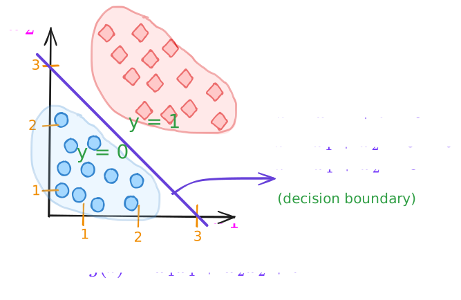
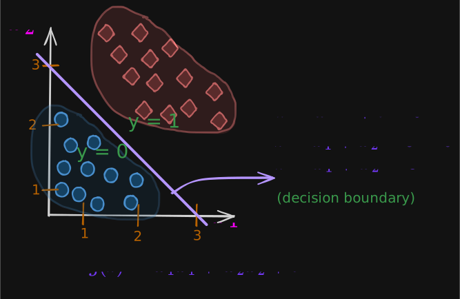
what we have just visualized is the decision boundary for logistic regression when the parameters w_1, w_2, and b are 1, 1, and −3.
Of course, if you had a different choice of the parameters, the decision boundary would be a different line.
Problem 2 - Non-Linear Decision Boundary
Now let’s look at a more complex example where the decision boundary is no longer a straight line.
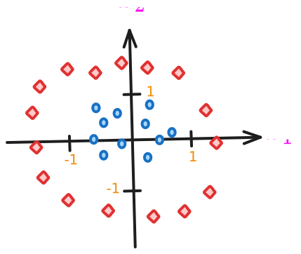
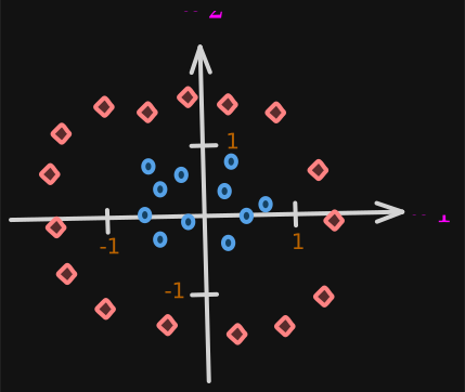
As before, diamonds denote the class y equals 1, and the little circles denote the class y equals 0.
We saw how to use polynomials in linear regression, and we can do the same in logistic regression.
Let’s use function:
therefore,
Let’s say, we ended up using and
So,
The decision boundary, as before, will correspond to when
That’s the decision boundary, and it looks like this:
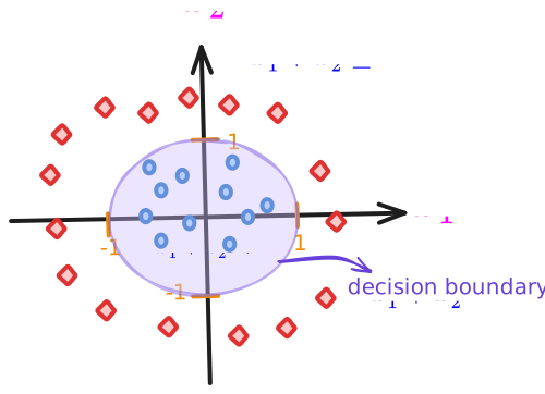
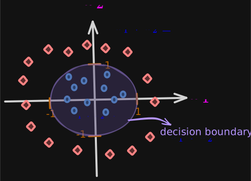
When , that’s this area outside the circle and that’s when you predict y to be 1.
Conversely, when , that’s this area inside the circle and that’s when you predict y to be 0.
Problem X - More Complex?
Can we come up with even more complex decision boundaries than these?
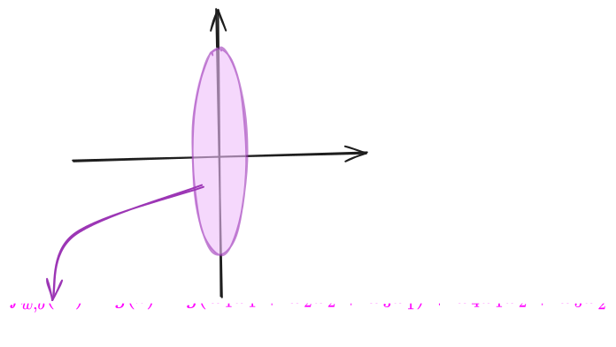
Yes, you can. You can do so by having even higher-order polynomial terms.
Ellipse
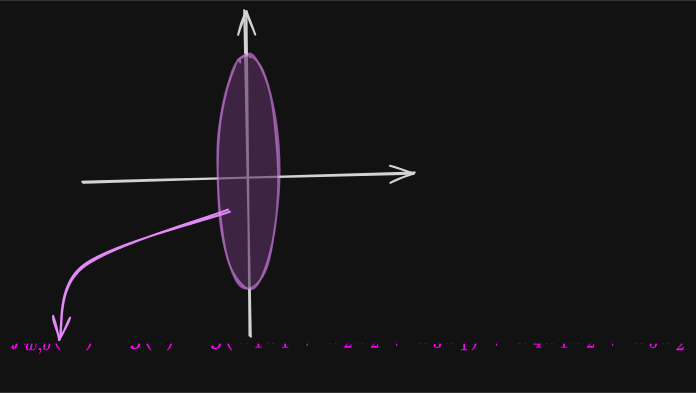
More Complex?
Yes!
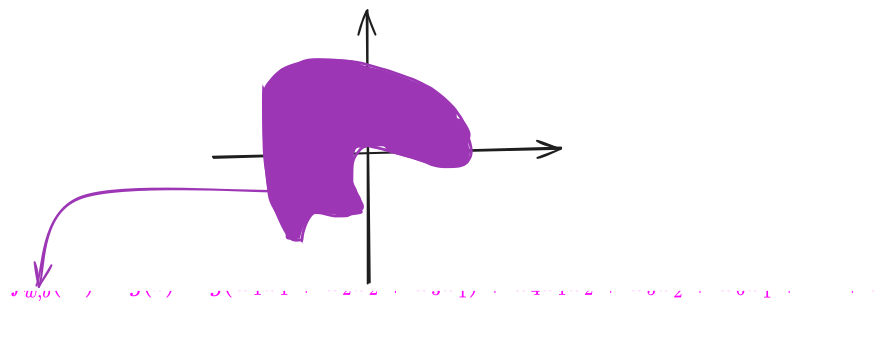
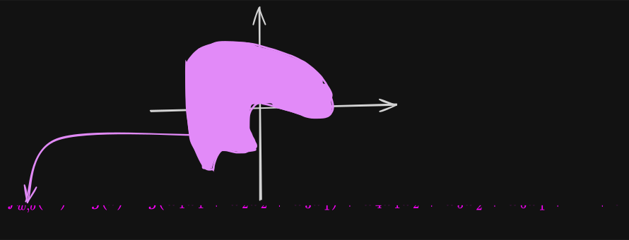
You can even get more complex decision boundaries, which can look like functions that look like this.
and even more complex!!!
This implementation of logistic regression will predict y equals 1 inside this shape and y equals 0 outside it.
With these polynomial features, you can get very complex decision boundaries. In other words, logistic regression can learn to fit pretty complex data.
Note: If you don’t include any higher-order polynomials, so the only features you use are , and so on, then the decision boundary will always be linear.
Cost Function
the cost function gives you a way to measure how well a specific set of parameters fits the training data.
This gives you a way to try to choose better parameters.
Logistic Regression is defined by this function:
The question you want to answer is, given a training set, how can you choose parameters
wandb?Let’s recall linear regression.
Why we can’t use mean squared error for classification?
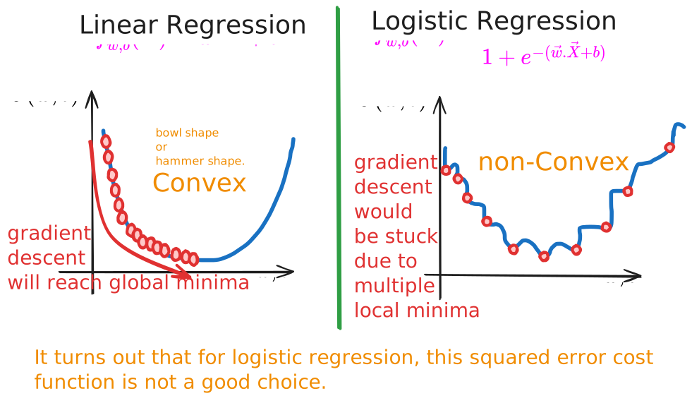
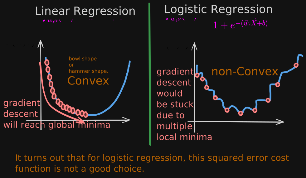
The non-linear nature of the model results in a “wiggly”, non-convex cost function with many potential local minima.
If using the mean squared error for logistic regression, the cost function is “non-convex”, so it’s more difficult for gradient descent to find an optimal value for the parameters w and b.
Different cost function!
Instead, there will be a different cost function that can make the cost function convex again. so gradient descent is guaranteed to converge to the global minimum.
NOTE: The only thing I’ve changed is that I put the one half inside the summation instead of outside the summation. This will make the math a little bit simpler.
Generalize Cost Function
I am going to generalize the cost function first:
where L = Loss Function.
Logistic Loss Function
By summing up the losses on all of the training examples, you get the cost function, which measures how well you’re doing on the entire training set.
y = 1
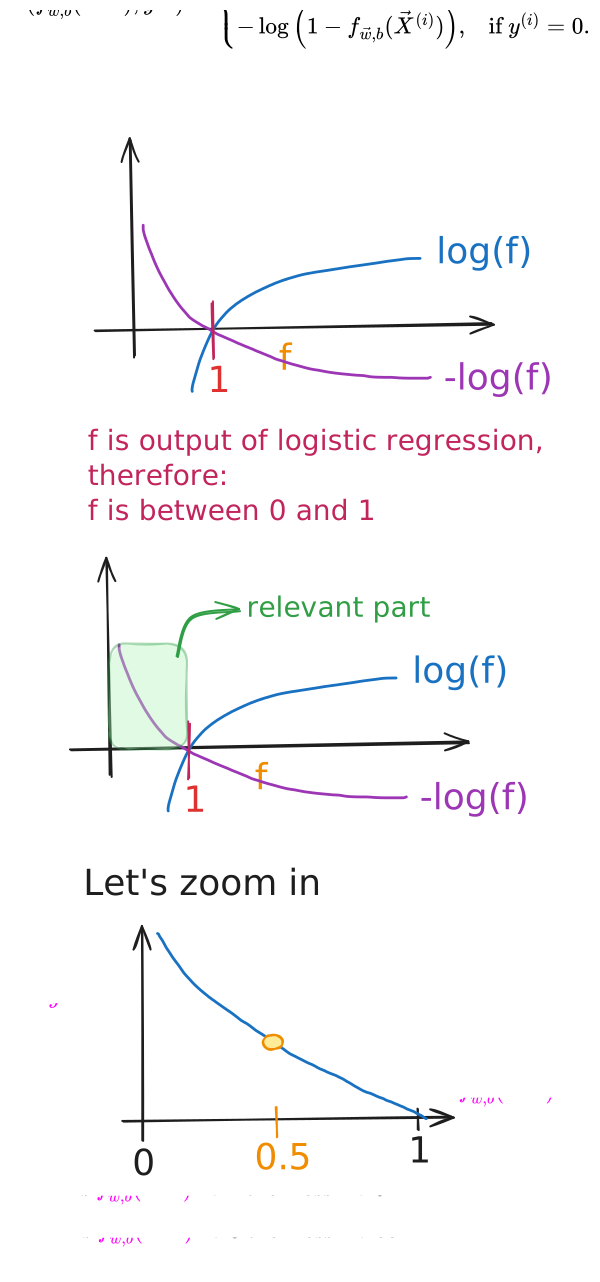
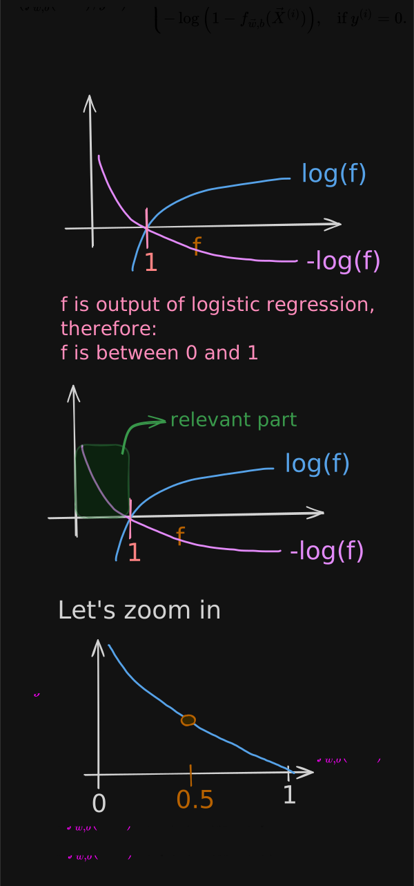
Let’s first consider the case of y equals 1 and plot what this function looks like to gain some intuition about what this loss function is doing.
y = 0
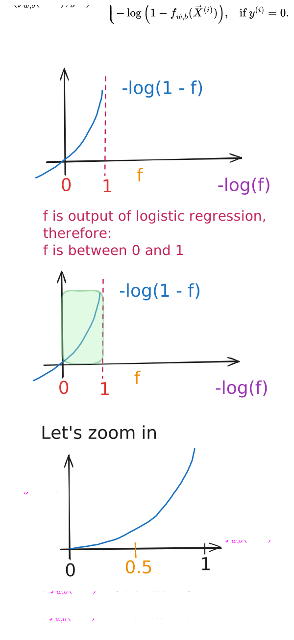
On this slide, let’s look at the second part of the loss function corresponding to when y is equal to 0.
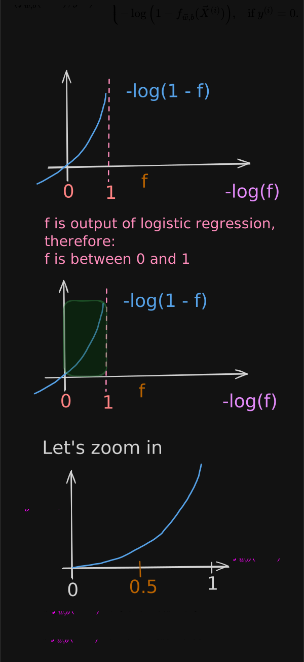
Coming back to our tumor dataset.
Going back to the tumor example: if the model predicts a 99.9% chance of malignancy, but it turns out not to be malignant (y = 0), then we penalize the model with a very high loss.
In this case of y equals 0, just as in the case of y equals 1 on the previous slide, the further the prediction f of x is away from the true value of y, the higher the loss.
***The Further the prediction is from target , the higher the loss. ***
the loss here actually goes really large and in fact approaches infinity.
When the true label is 1, the algorithm is strongly incentivized not to predict something too close to 0.
the overall cost function will be convex and thus you can reliably use gradient descent to take you to the global minimum.
Convex is better
the overall cost function will be convex and thus you can reliably use gradient descent to take you to the global minimum.
Learn to prove if cost function is convex
find w, b that minimize cost J.
Simplified Cost Function for Logistic Regression
Here is the Loss Function for Logistic Regression:
Because we’re still working on a binary classification problem, y is either zero or one. Because y is either zero or one and cannot take on any value other than zero or one, we’ll be able to come up with a simpler way to write this loss function. You can write the loss function as follows:
Test for y = 1
if :
Test for y = 0
if :
What you see is that whether y is one or zero, this single expression here is equivalent to the more complex expression up here, which is why this gives us a simpler way to write the loss with just one equation without separating out these two cases, like we did on top.
Let’s Write Cost Function
Loss Function:
Cost Function:
Therefore, the Cost Function for Logistic Regression is:
This is the cost function that pretty much everyone uses.
I’d just like to mention that this particular cost function is derived from statistics using a statistical principle called maximum likelihood estimation, which is an idea from statistics on how to efficiently find parameters for different models.
NOTE:
Loss is calculated per training example
Cost is calculated over all training examples
Gradient Descent for Logistic Regression
To fit the parameters of a logistic regression model, we’re going to try to find the values of the parameters w and b that minimize the cost function J of w and b, and we’ll again apply gradient descent to do this.
Here is the Cost Function:
To minimize the cost function, we use gradient descent:
for ; where is the number of features.
if we solve the partial derivatives:
and
NOTE: use simultaneous updates, meaning that you first compute the right-hand side for all of these updates and then simultaneously overwrite all the values on the left at the same time.
Gradient Descent For Logistic Regression
Now, one funny thing you might be wondering is, that’s weird. These two equations look exactly like the ones we had come up with previously for linear regression so you might be wondering, is linear regression actually secretly the same as logistic regression?
Well, even though these equations look the same, the reason that this is not linear regression is because the definition for the function f of x has changed.
For Linear Regression:
For Logistic Regression:
Although the algorithm written looks the same for both linear regression and logistic regression, actually they’re two very different algorithms because the definition for f of x is not the same.
Same Concepts as Linear Regression
Monitor Gradient Descent (Learning Curve)
Vectorized Implementation
Feature Scaling
Feature scaling applied the same way to scale the different features to take on similar ranges of values can also speed up gradient descent for logistic regression.