In this chapter, we build linear regression from scratch: first with a single feature, then with multiple features. Along the way, we will see how the model’s parameters, the cost function, and gradient descent work together, and develop the intuition behind each one before turning it into code.
Regression model is predicting a number.
Types of Regression:
Linear Regression Model
Polynomial Regression Model
Architecture
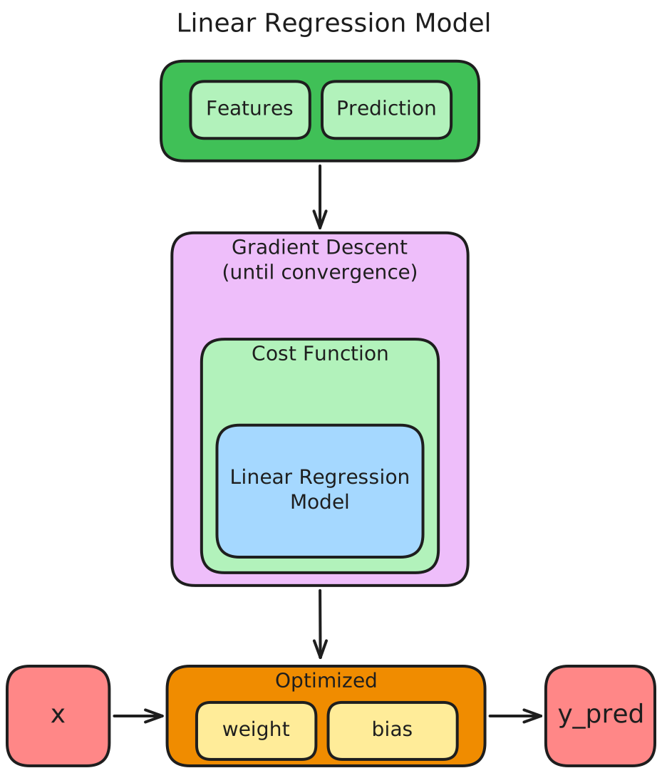
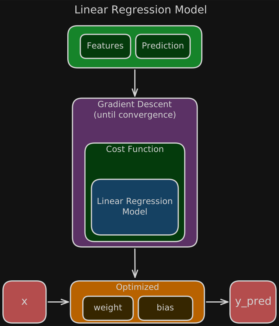
Linear Regression Model
Cost Function
here, L is loss function. We can write outside of summation to generalize. I have kept it with Loss function. So in general, the above equation can also be written as:
Gradient Descent
where,
= weights,
= bias,
= features,
= target / output,
= prediction,
= Loss Function,
= Cost Function
= Regularization of
Linear Regression Model with Single Feature
Linear Regression Model is fitting a straight line to the data.
Problem that we can address with Linear Regression Problem is: We want to predict the price of a house based on the size of the house.
Here we have a graph where the horizontal axis is the size of the house in square feet, and the vertical axis is the price of a house in thousands of dollars.
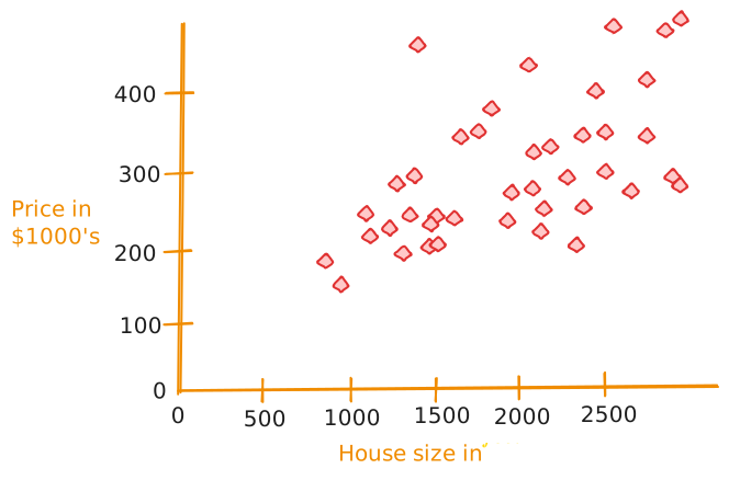
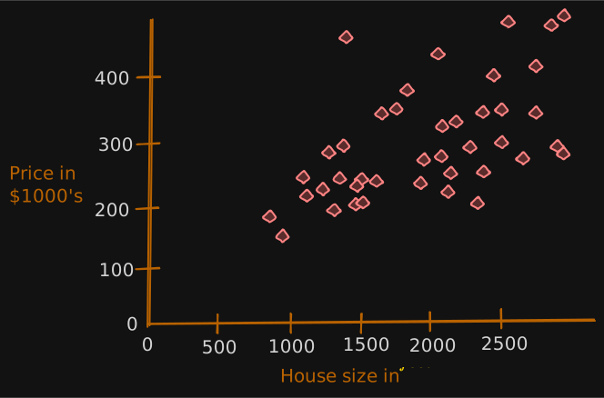
Now, let’s say you’re a real estate agent and you’re helping a client to sell her house. She is asking you, how much do you think I can get for this house?
This dataset might help you estimate the price she could get for it. You start by measuring the size of the house, and it turns out that the house is 1250 square feet. How much do you think this house could sell for?
One thing you could do this, you can build a linear regression model from this dataset.
Your model will fit a straight line to the data, which might look like this.
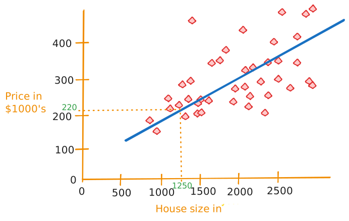
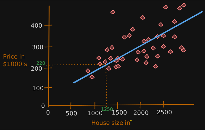
Based on this straight line fit to the data, you can see that the house is 1250 square feet, it will intersect the best fit line over here, and if you trace that to the vertical axis on the left, you can see the price is maybe around here, say about $220,000.
This is the example of Regression Problem of the Supervised Learning Model.
In addition to visualizing this data as a plot here on the left, there’s one other way of looking at the data that would be useful, and that’s a data table here on the right.
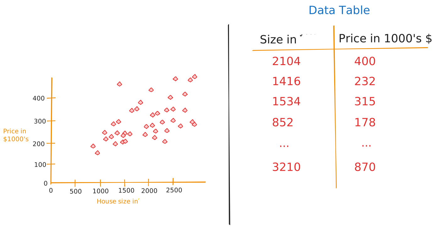
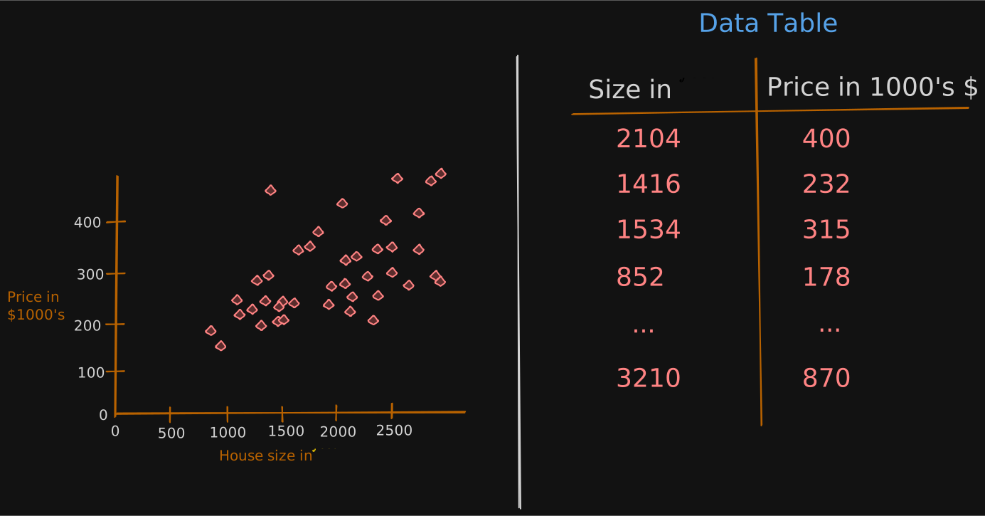
The data comprises a set of inputs. This would be the size of the house, and It also has outputs.
If we have 47 rows in this data table, than we would have 47 diamonds in the plot.
Process
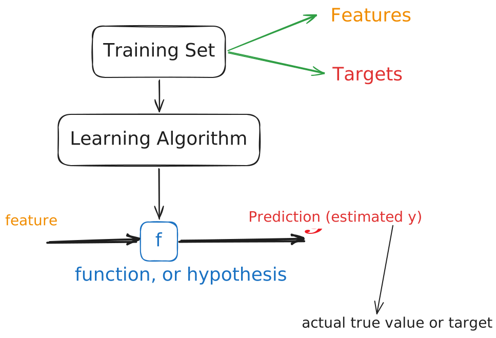
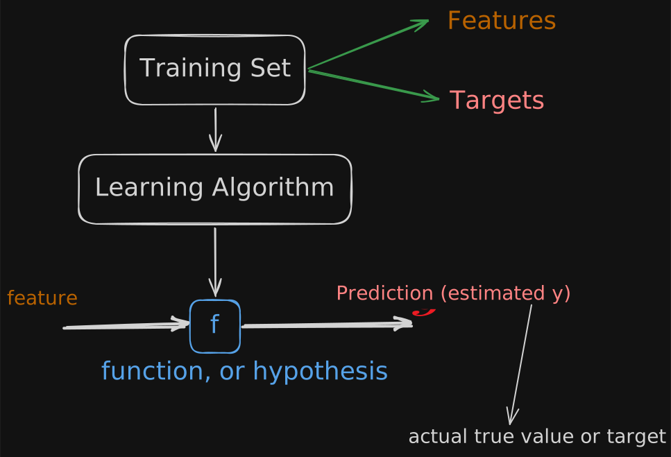
A training set in supervised learning includes both the input features, such as the size of the house and also the output targets, such as the price of the house. The output targets are the right answers to the model we’ll learn from.
To train the model, you feed the training set, both the input features and the output targets to your learning algorithm. Then your supervised learning algorithm will produce some function.
We’ll write this function as lowercase
f, wherefstands for function. Historically, this function used to be called a hypothesis.The job with f is to take a new input x and output and estimate or a prediction, (“y-hat”). In machine learning, the convention is that y-hat is the estimate or the prediction for y. The function f is called the model. X is called the input or the input feature, and the output of the model is the prediction, y-hat. The model’s prediction is the estimated value of y.
When the symbol is just the letter y, then that refers to the target, which is the actual true value in the training set. In contrast, y-hat is an estimate. It may or may not be the actual true value.
Well, if you’re helping your client to sell the house, well, the true price of the house is unknown until they sell it. Your model f, given the size, outputs the price which is the estimator, that is the prediction of what the true price will be.
Now, when we design a learning algorithm, a key question is, how are we going to represent the function f? Or in other words, what is the math formula we’re going to use to compute f?
For now, let’s stick with f being a straight line.
Your function can be written as:
where w, and b are numbers representing weight and bias which determine the prediction y-hat based on the input feature X.
means f is a function that takes X as input, and depending on the values of w and b, f will output some value of a prediction y-hat.
As an alternative to writing this, , we can sometimes write it as .
Let’s plot the training set on the graph where the input feature X is on the horizontal axis and the output target y is on the vertical axis. Remember, the algorithm learns from this data and generates the best-fit line.
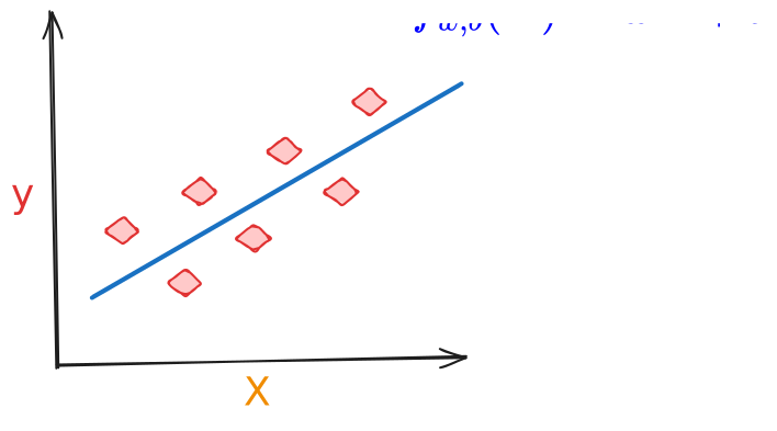
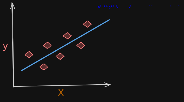
is making predictions for the value of y using a straight-line function of X.
You may ask, why are we choosing a linear function, where linear function is just a fancy term for a straight line instead of some non-linear function like a curve or a parabola? Well, sometimes you want to fit more complex non-linear functions as well, like a curve like this.
This particular model has a name. It’s called Linear Regression. More specifically, it’s Linear Regression with one variable where the phrase one variable means that there’s a single input variable or feature X, namely the size of the house. Another name for a linear model with one input variable is univariate linear regression, where uni means one in Latin, and where variate means variable.
Cost Function
The cost function tells us how well the model is doing so that we can try to get it to do better.
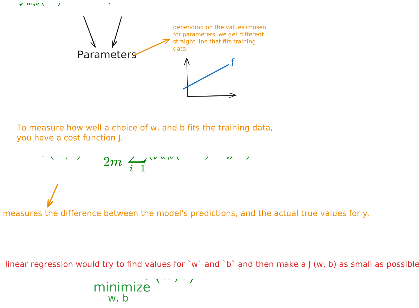
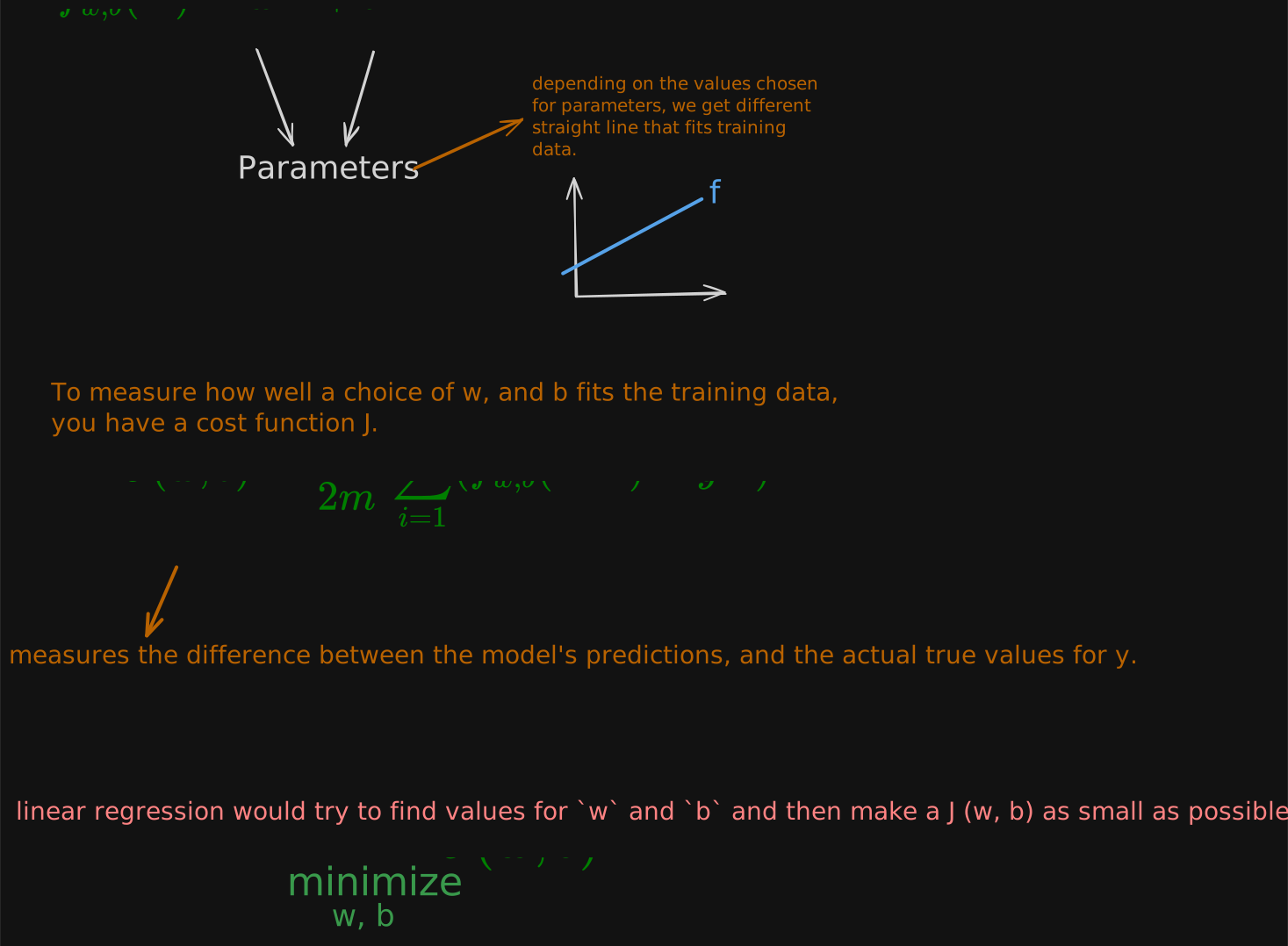
Depending on the values you’ve chosen for
wandbyou get a different function , also written as , which generates a different line on the graph.
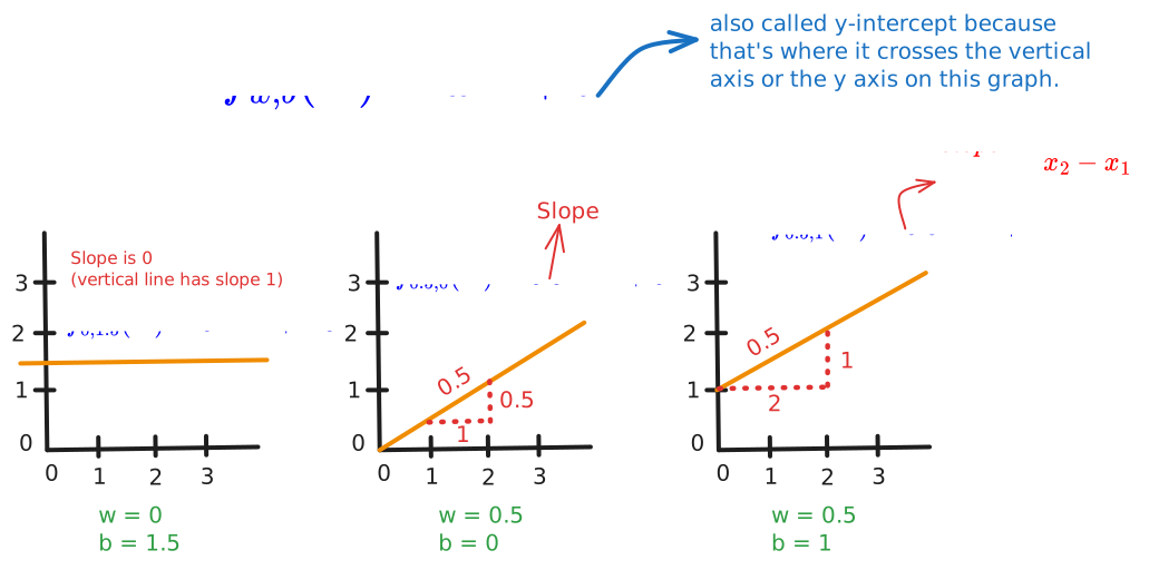
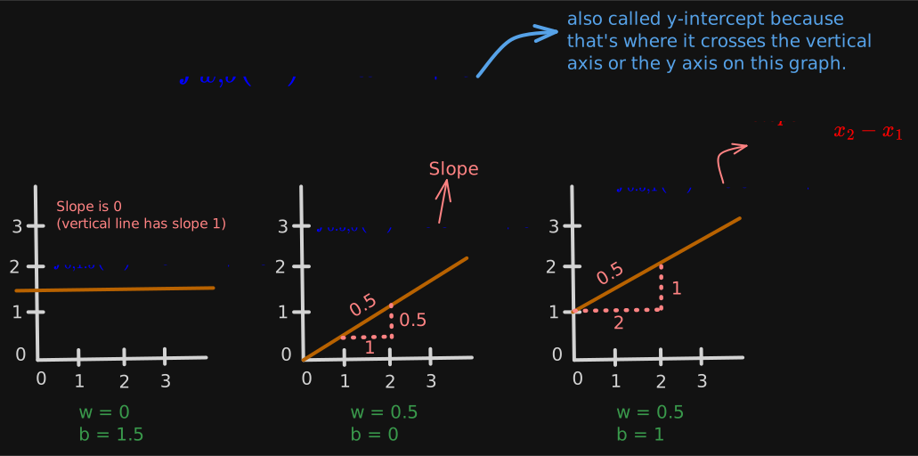
Recall that you have a training set like the one shown here.
With linear regression, what you want to do is to choose values for the parameters w and b so that the straight line you get from the function f somehow fits the data well. Like maybe this line shown here. When I see that the line fits the data visually, you can think of this to mean that the line defined by f is roughly passing through or somewhere close to the training examples as compared to other possible lines that are not as close to these points.
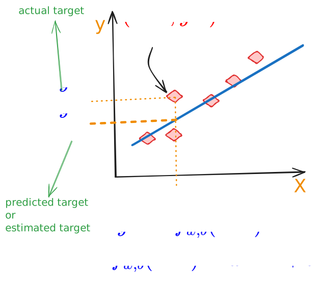
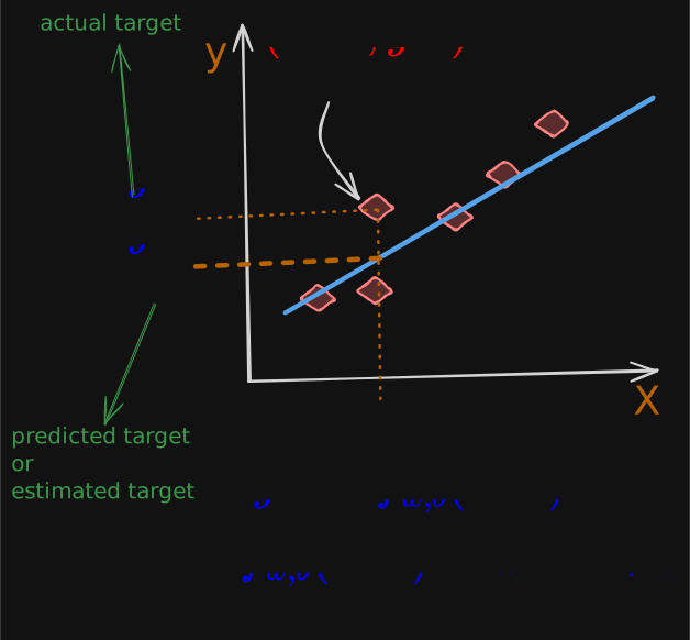
Now the question is how do you find values for
wandbso that the prediction is close to the true target for many or maybe all training examples .Find w,b: is close to for all
To answer that question, let’s first take a look at how to measure how well a line fits the training data. To do that, we’re going to construct a cost function.
The cost function takes the prediction y hat and compares it to the target y by taking y hat minus y. This difference is called the error, we’re measuring how far off to prediction is from the target. Next, let’s computes the square of this error. Also, we’re going to want to compute this term for different training examples i in the training set. When measuring the error, for example i, we’ll compute this squared error term. Finally, we want to measure the error across the entire training set. In particular, let’s sum up the squared errors like this. We’ll sum from i equals 1,2, 3 all the way up to m and remember that m is the number of training examples, which is 47 for this dataset. Notice that if we have more training examples m is larger and your cost function will calculate a bigger number. This is summing over more examples. To build a cost function that doesn’t automatically get bigger as the training set size gets larger by convention, we will compute the average squared error instead of the total squared error and we do that by dividing by m like this. We’re nearly there. Just one last thing.
By convention, the cost function that machine learning people use actually divides by 2 times m. The extra division by 2 is just meant to make some of our later calculations look neater, but the cost function still works whether you include this division by 2 or not.
Mathematically,
where m = number of training examples.
This expression right here is the cost function and we’re going to write to refer to the cost function.
Therefore, cost function is
This is also called the squared error cost function, and it’s called this because you’re taking the square of these error terms.
Just as a reminder, the prediction is equal to the outputs of the model . We can rewrite the cost function as
In machine learning different people will use different cost functions for different applications, but the squared error cost function is by far the most commonly used one for linear regression and for that matter, for all regression problems where it seems to give good results for many applications.
Intuition
What does mean when it’s larger or smaller? How does the cost function make an impact?
Simplified (bias = 0)
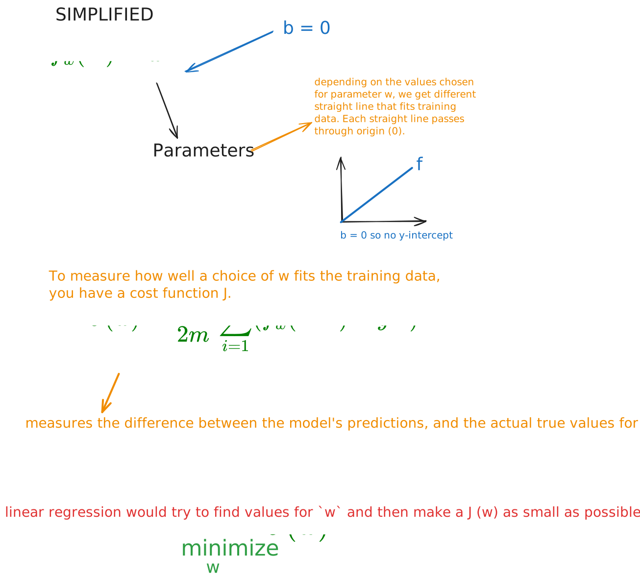
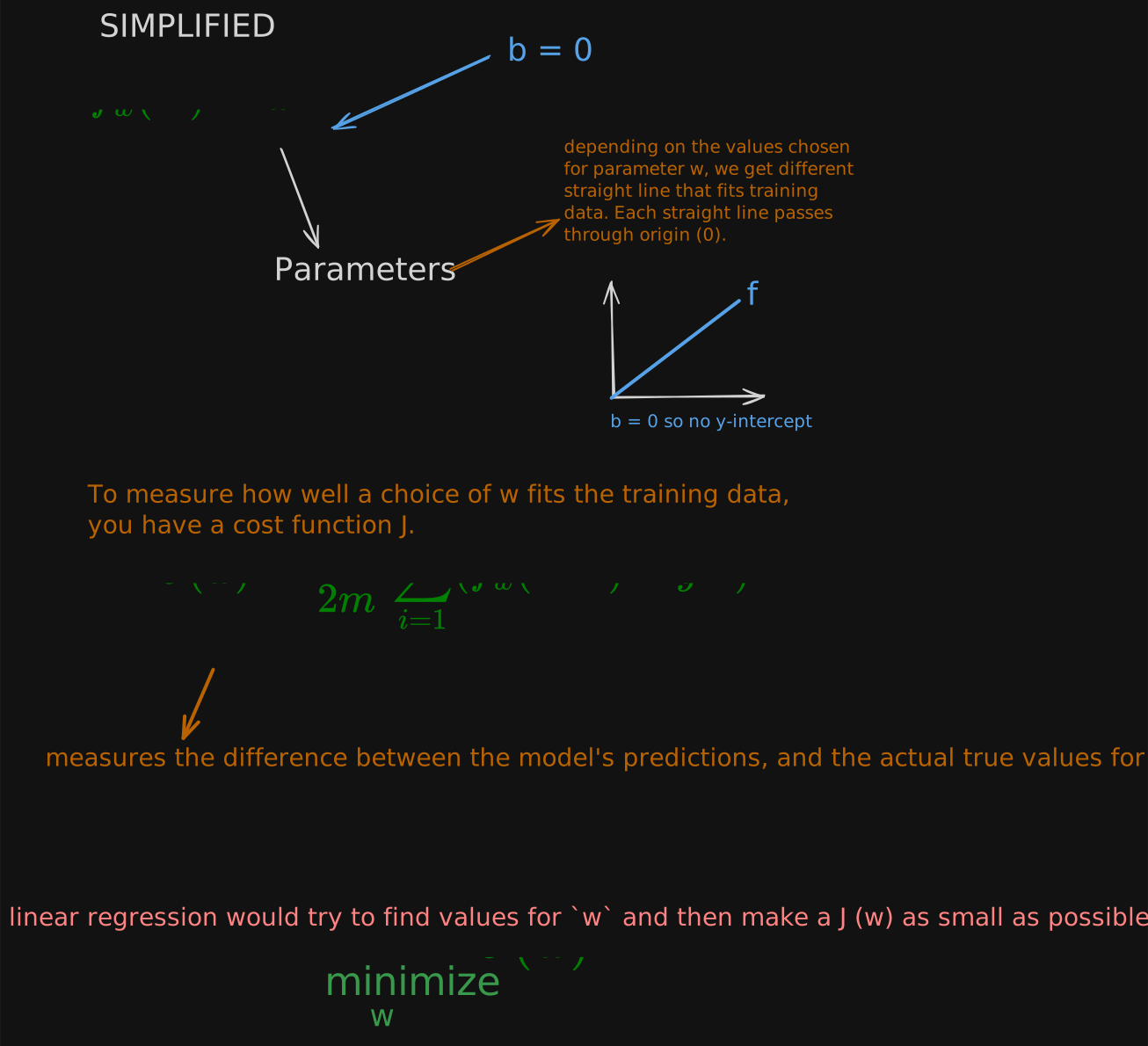
Now, in order for us to better visualize the , let’s work with a simplified version of the linear regression model.
let’s see how the cost function changes as you choose different values for the parameter
w. In particular, let’s look at graphs of the model , and the cost function .First, notice that for f subscript w, when the parameter w is fixed, that is, is always a constant value, then is only a function of X, which means that the estimated value of y depends on the value of the input X.
In contrast, looking to the right, the , is a function , where w controls the slope of the line defined by . The cost defined by J, depends on a parameter, in this case, the parameter w.
therefore:
- for fixed w, function of X; X is input
- function of w; w is parameter
Let’s see how w impacts cost function for different w
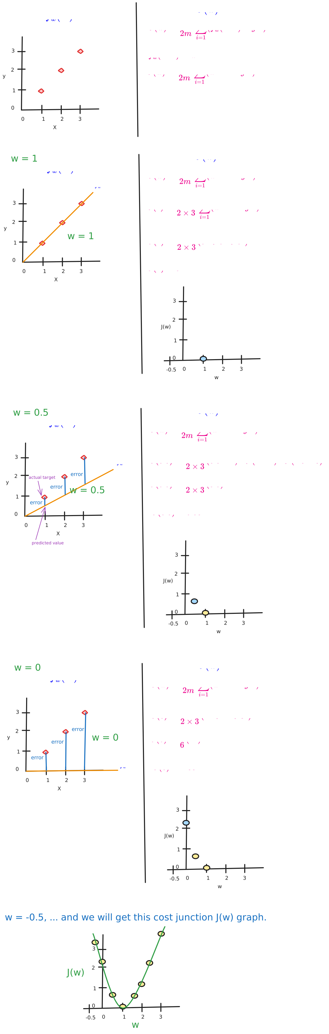
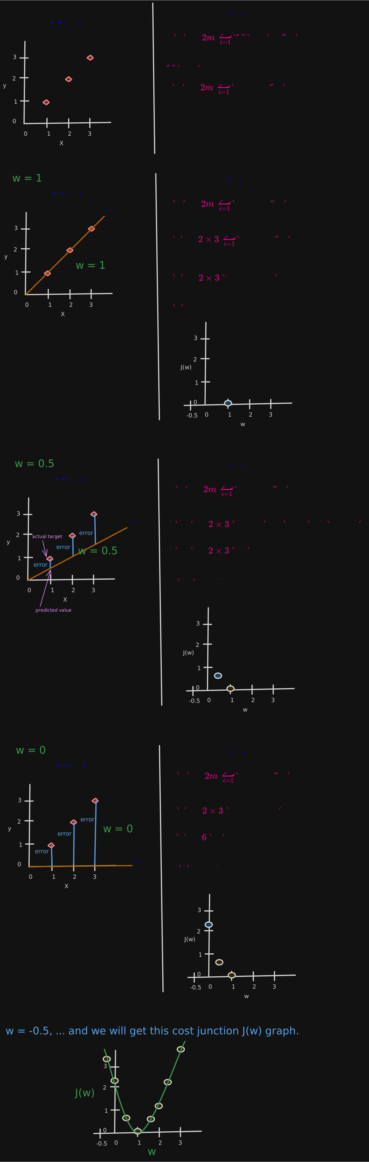
Each value of parameter w corresponds to different straight line fit, , on the graph to the left.
For each value of w you wind up with a different line and its corresponding costs, , and you can use these points to trace out this plot.
Given this, how can you choose the value of w that results in the function f, fitting the data well? Well, as you can imagine, choosing a value of w that causes to be as small as possible seems like a good bet. J is the cost function that measures how big the squared errors are, so choosing w that minimizes these squared errors, makes them as small as possible, will give us a good model.
In this example, choosing
w = 1is a great bet.
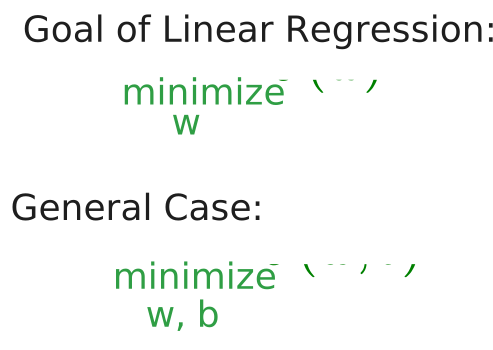
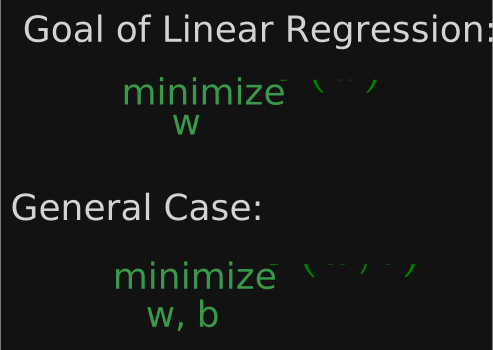
In the more general case where we had parameters w and b rather than just w, you find the values of w and b that minimize J.
Solution to Exercise 3.1
d. When the cost is at or near a minimum.
Explaination: The goal of linear regression is to find the parameters w or w and b that results in the smallest possible value for the .
The goal of linear regression is to find the parameters w or w and b that results in the smallest possible value for the .
Full Version
In simplified version, we set b = 0. Now, let’s go back to the original model with both parameters w and b without setting b to be equal to 0.
Here is the training dataset:
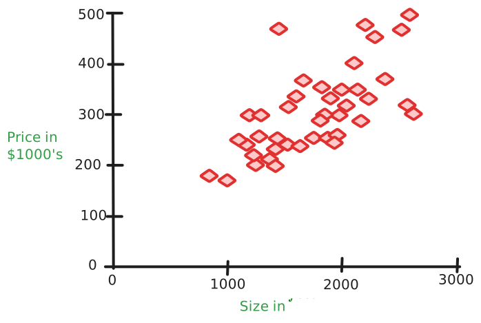
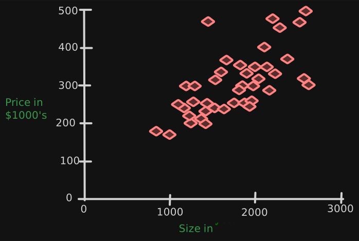
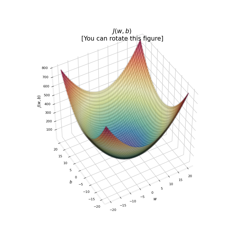
When we had only one parameter, w, the cost function had this U-shaped curve, shaped a bit like a soup bowl. Now, in this housing price example that we have on this slide, we have two parameters, w and b. The plots becomes a little more complex. It turns out that the cost function also has a similar shape like a soup bowl, except in three dimensions instead of two.
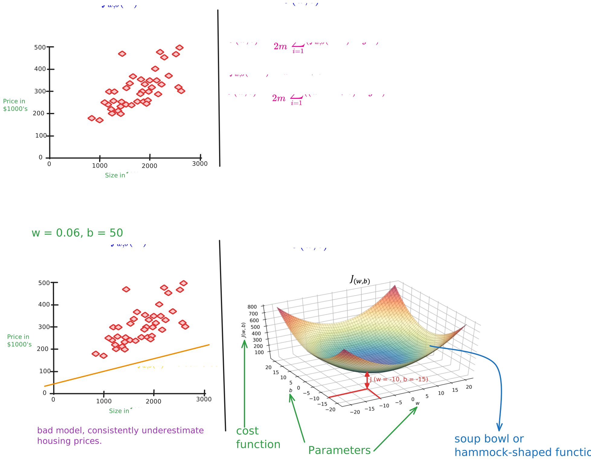
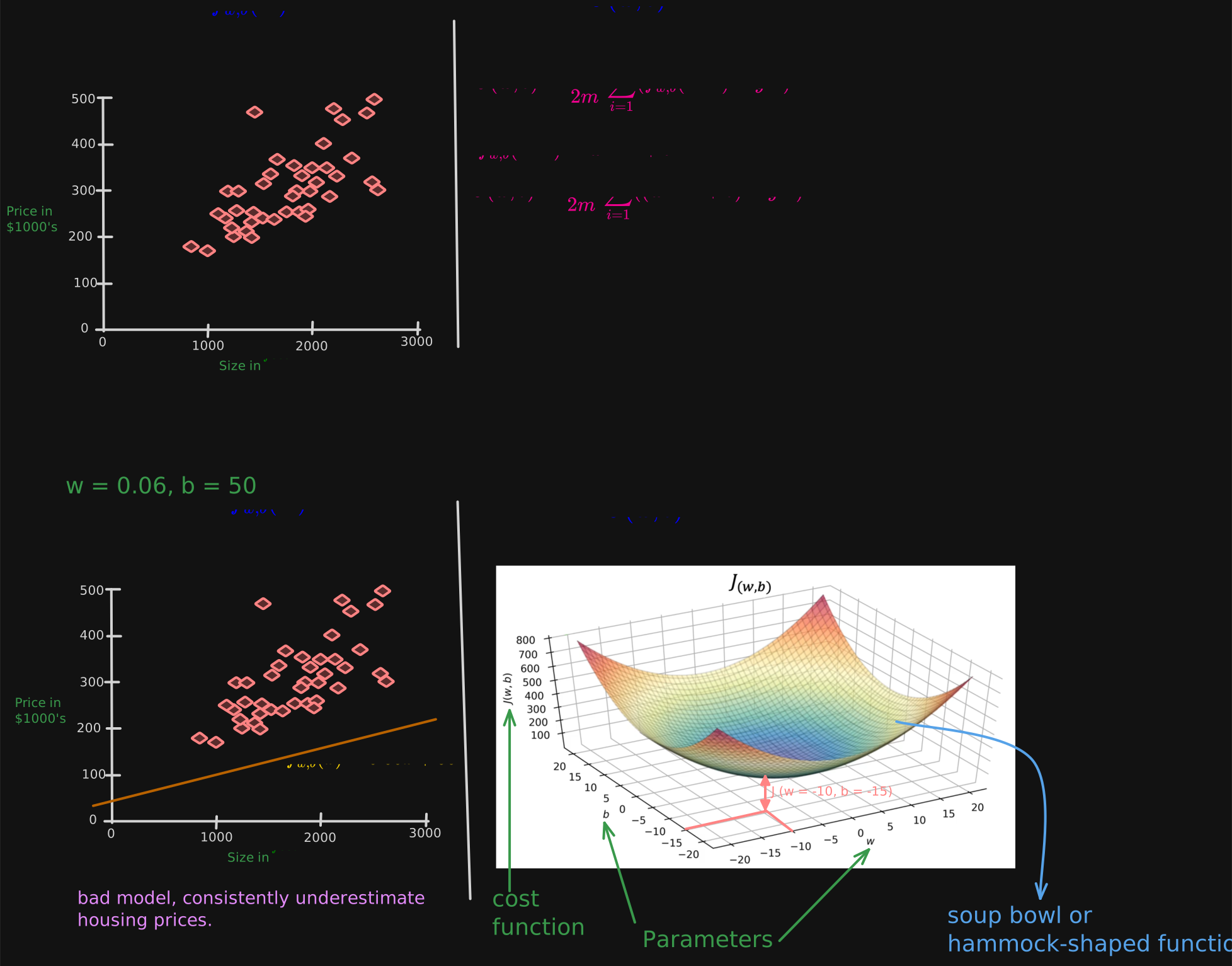
here’s another way of plotting the that would be useful for visualization, which is, rather than using these 3D-surface plots, and plot it using something called a contour plot.
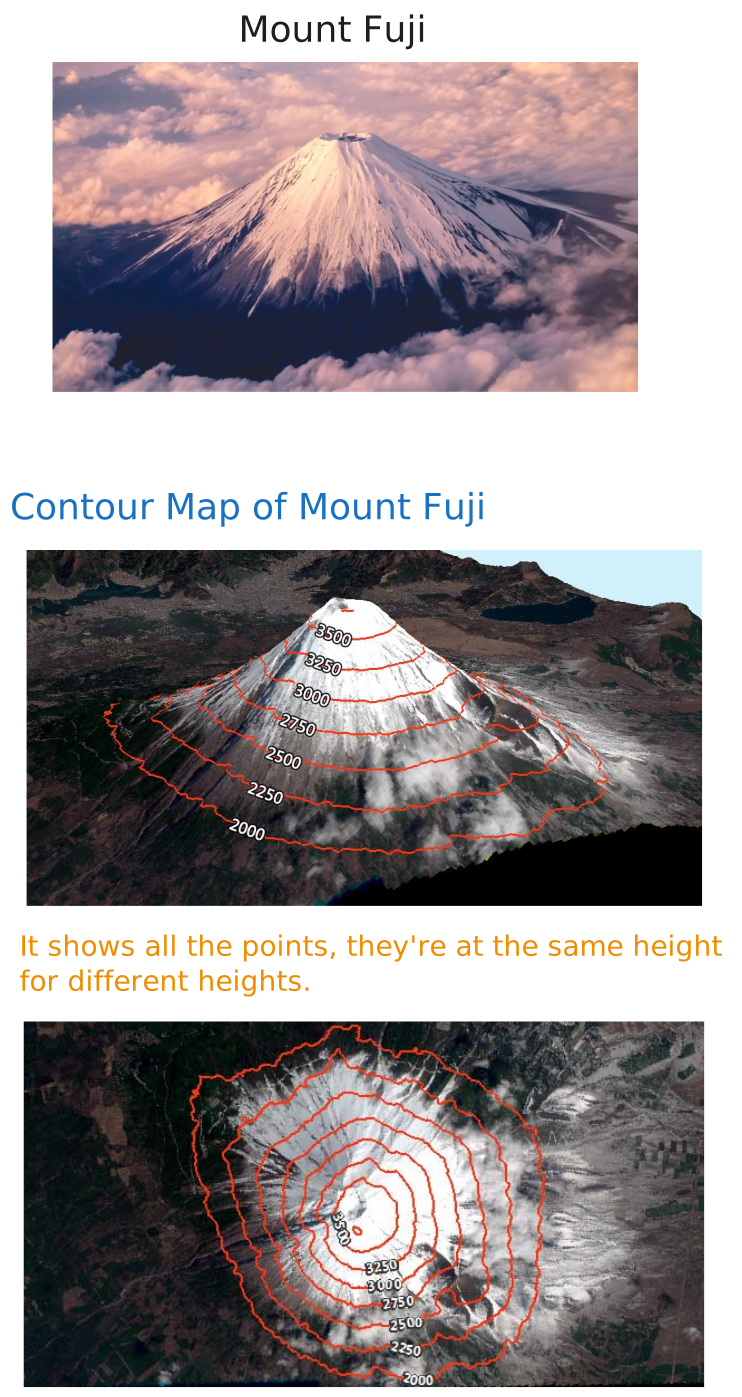
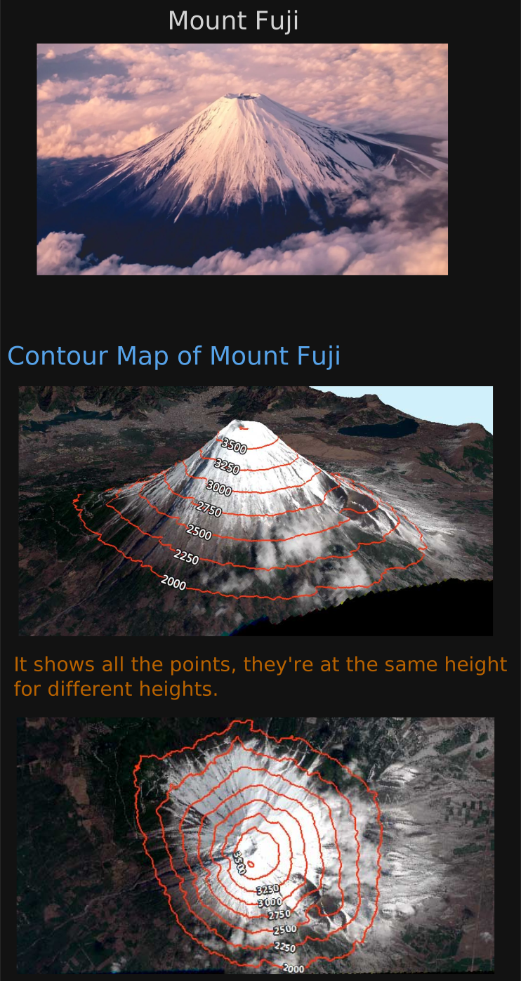
If you’ve ever seen a topographical map showing how high different mountains are, the contours in a topographical map are basically horizontal slices of the landscape of say, a mountain.
Contour Map of Mount Fuji.
here on the upper right is a contour plot of this exact same cost function as that shown at the bottom. The two axes on this contour plots are b, on the vertical axis, and w on the horizontal axis. What each of these ovals, also called ellipses, shows, is the center points on the 3D surface which are at the exact same height.
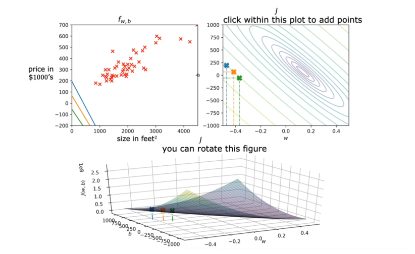
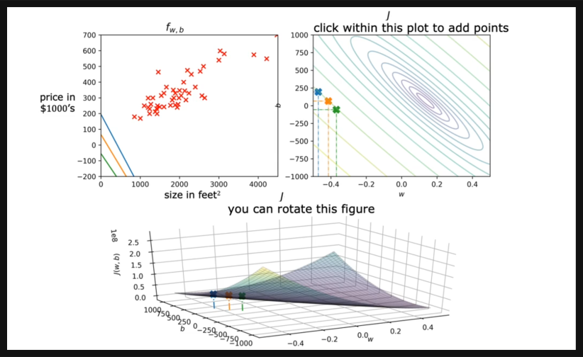
In other words, the set of points which have the same value for the .
To get the contour plots, you take the 3D surface at the bottom and you use a knife to slice it horizontally. You take horizontal slices of that 3D surface and get all the points, they’re at the same height. Therefore, each horizontal slice ends up being shown as one of these ellipses or one of these ovals. Concretely, if you take that point, and that point, and that point, all of these three points have the same value for the , even though they have different values for w and b.
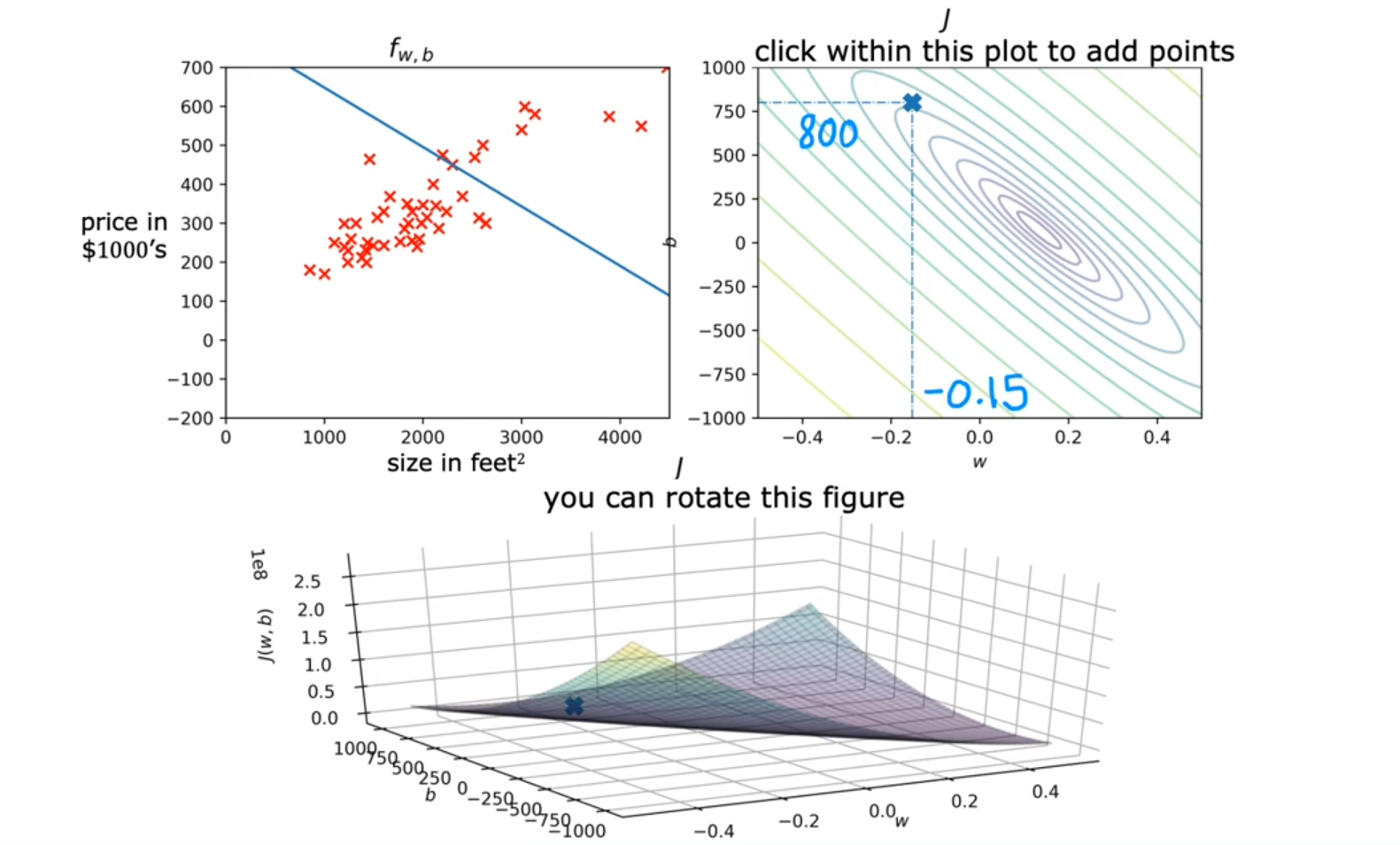
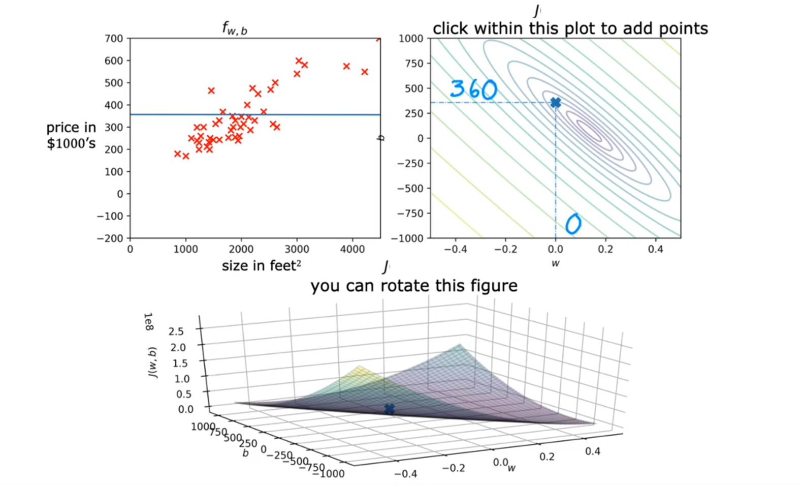
In the figure on the upper left, you see also that these three points correspond to different functions, f, all three of which are actually pretty bad for predicting housing prices in this case. Now, the bottom of the bowl, where the is at a minimum, is this point right here, at the center of this concentric ovals.
It turns out that the contour plots are a convenient way to visualize the 3D , but plotted in just 2D.
Remember that the minimum is at the center of that smallest ellipse.
Let’s look at some of the important visualization on our house price dataset.
w = -0.15 and b = 800
w = 0 and b = 360
w = 0.13 and b = 71
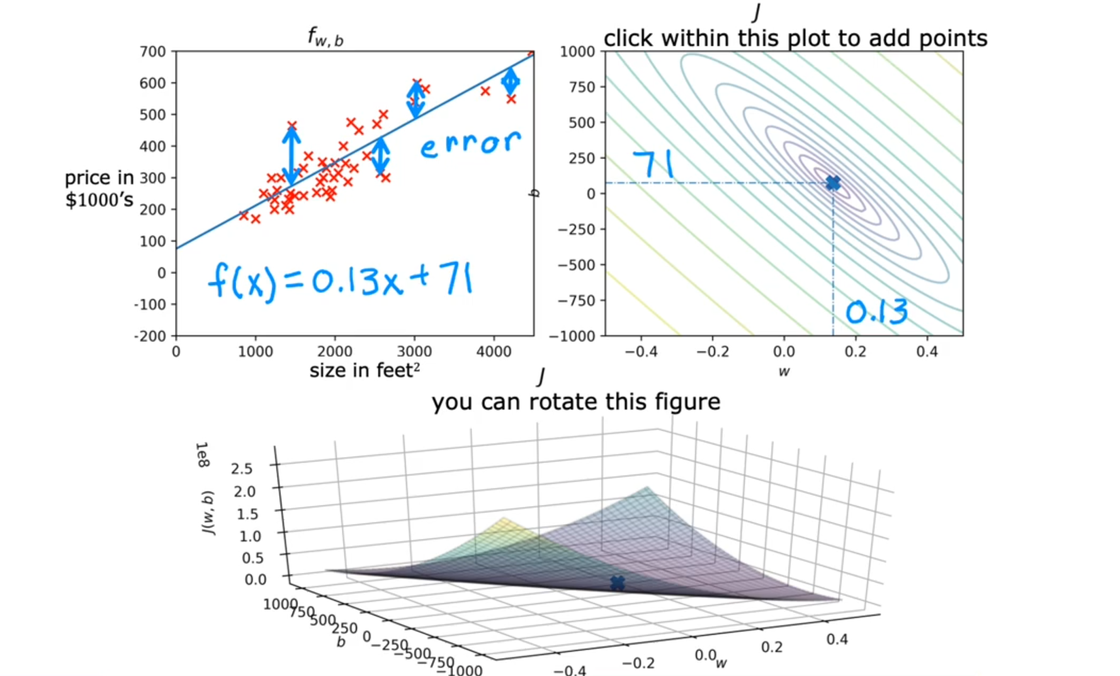
this looks like a pretty good fit to the training set. You can see on the right, this point representing the cost is very close to the center of the smaller ellipse, it’s not quite exactly the minimum, but it’s pretty close.
I hope that by looking at these figures, you can get a better sense of how different choices of the parameters affect the line f of X and how this corresponds to different values for the cost j, and hopefully you can see how the better fit lines correspond to points on the graph of j that are closer to the minimum possible cost for this cost function .
Now in linear regression, rather than having to manually try to read a contour plot for the best value for w and b, which isn’t really a good procedure and also won’t work once we get to more complex machine learning models. What you really want is an efficient algorithm that you can write in code for automatically finding the values of parameters w and b they give you the best fit line. That minimizes the . There is an algorithm for doing this called gradient descent.
The fact that the cost function squares the loss ensures that the ‘error surface’ is convex like a soup bowl. It will always have a minimum that can be reached by following the gradient in all dimensions
Gradient Descent
This algorithm is one of the most important algorithms in machine learning. Gradient descent and variations on gradient descent are used to train, not just linear regression, but some of the biggest and most complex models in all of AI.
It would be nice if we had a more systematic way to find the values of w and b, that results in the smallest possible cost, . It turns out there’s an algorithm called gradient descent that you can use to do that.
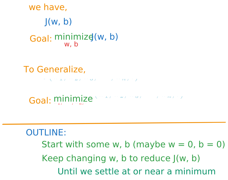
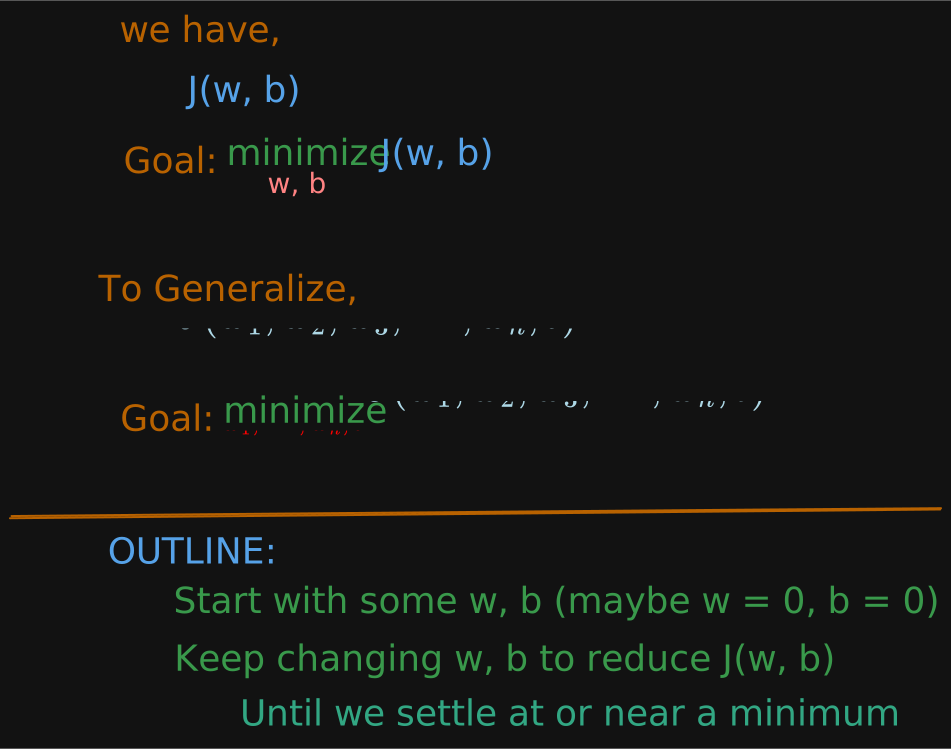
Overview:
You have the cost function that you want to minimize.
gradient descent is an algorithm that you can use to try to minimize any function, not just a cost function for linear regression.
For instance, if you have a cost function J as a function of up to and b, your objective is to minimize over the parameters to and . In other words, you want to pick values for through and , that gives you the smallest possible value of . It turns out that gradient descent is an algorithm that you can apply to try to minimize this cost function as well.
What you’re going to do is just to start off with some initial guesses for w and b. In linear regression, it won’t matter too much what the initial value are, so a common choice is to set them both to 0.
For example, you can set w to 0 and b to 0 as the initial guess.
With the gradient descent algorithm, what you’re going to do is, you’ll keep on changing the parameters and a bit every time to try to reduce the cost until hopefully settles at or near a minimum.
One thing I should note is that for some functions j that may not be a bowl shape or a hammock shape, it is possible for there to be more than one possible minimum.
Overview:
Example of Gradient Descent - Moving Down the Hill
Let’s take a look at an example of a more complex surface plot j to see what gradient is doing.
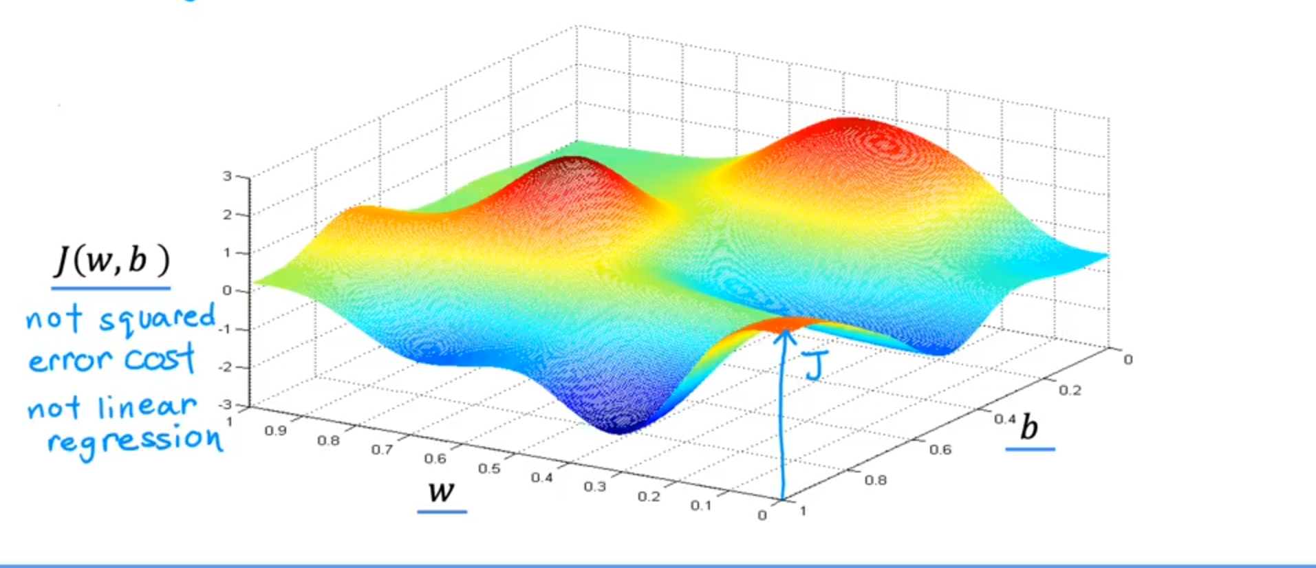
This function is not a squared error cost function.
For linear regression with the squared error cost function, you always end up with a bowl shape or a hammock shape. But this is a type of cost function you might get if you’re training a neural network model.
Notice the axes, that is w and b on the bottom axis. For different values of w and b, you get different points on this surface, , where the height of the surface at some point is the value of the cost function.
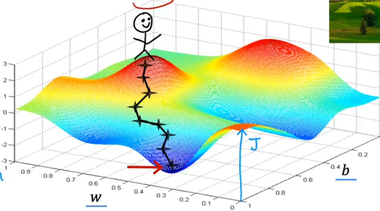
Now, let’s imagine that this surface plot is actually a view of a slightly hilly outdoor park or a golf course where the high points are hills and the low points are valleys like so. I’d like you to imagine if you will, that you are physically standing at this point on the hill. If it helps you to relax, imagine that there’s lots of really nice green grass and butterflies and flowers is a really nice hill.
Your goal is to start up here and get to the bottom of one of these valleys as efficiently as possible.
What the gradient descent algorithm does is, you’re going to spin around 360 degrees and look around and ask yourself, if I were to take a tiny little baby step in one direction, and I want to go downhill as quickly as possible to or one of these valleys. What direction do I choose to take that baby step?
Well, if you want to walk down this hill as efficiently as possible, it turns out that if you’re standing at this point in the hill and you look around, you will notice that the best direction to take your next step downhill is roughly that direction.
Mathematically, this is the direction of steepest descent. It means that when you take a tiny baby little step, this takes you downhill faster than a tiny little baby step you could have taken in any other direction. After taking this first step, you’re now at this point on the hill over here.
Now let’s repeat the process.
Standing at this new point, you’re going to again spin around 360 degrees and ask yourself, in what direction will I take the next little baby step in order to move downhill? If you do that and take another step, you end up moving a bit in that direction and you can keep going. From this new point, you can again look around and decide what direction would take you downhill most quickly. Take another step, another step, and so on, until you find yourself at the bottom of this valley, at this local minimum, right here.
What you just did was go through multiple steps of gradient descent. It turns out, gradient descent has an interesting property.
Remember that you can choose a starting point at the surface by choosing starting values for the parameters w and b.
Now, imagine if you try gradient descent again, but this time you choose a different starting point by choosing parameters that place your starting point just a couple of steps to the right over here. If you then repeat the gradient descent process, which means you look around, take a little step in the direction of steepest descent so you end up here. Then you again look around, take another step, and so on. If you were to run gradient descent this second time, starting just a couple steps in the right of where we did it the first time, then you end up in a totally different valley. This different minimum over here on the right.
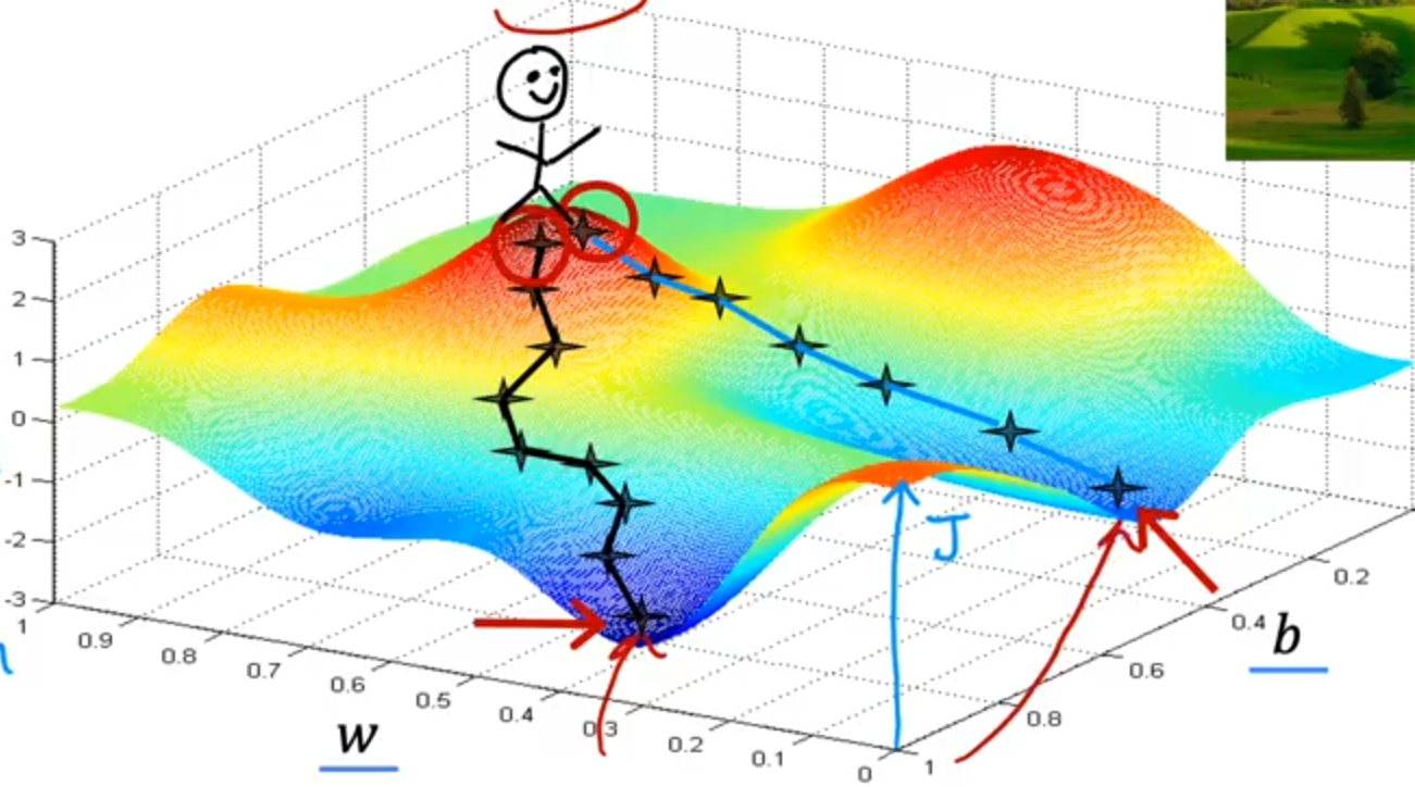
The bottoms of both the first and the second valleys are called local minima. Because if you start going down the first valley, gradient descent won’t lead you to the second valley, and the same is true if you started going down the second valley, you stay in that second minimum and not find your way into the first local minimum. This is an interesting property of the gradient descent algorithm.
Gradient Descent Algorithm & Its Implementation
let’s look at the mathematical expressions that you can implement to make gradient descent work.
Algorithm
Below is the equations after solving the derivatives using calculus.
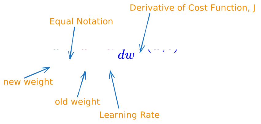
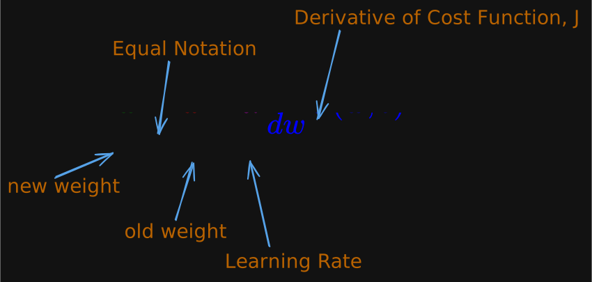
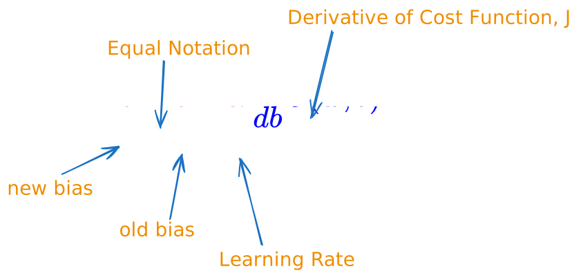
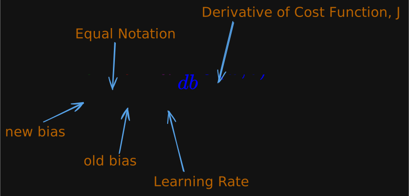
(Equals): It equals the right hand side of the equation to the left hand side.
It’s not a comparison; it’s an assignment.
(Alpha) : The learning rate is usually a small positive number between 0 and 1 and it might be say, 0.01. The learning rate controls how big of a step you take when updating the model’s parameters, w and b.
If Alpha is very large, then that corresponds to a very aggressive gradient descent procedure where you’re trying to take huge steps downhill.
If Alpha is very small, then you’d be taking small baby steps downhill.
or (derivative term of the ): this derivative term tells you in which direction you want to take your baby step.
or : In combination with the learning rate Alpha, it also determines the size of the steps you want to take downhill.
Remember in the graph of the surface plot where you’re taking baby steps until you get to the bottom of the valley, well, for the gradient descent algorithm, you’re going to repeat these two update steps until the algorithm converges.
By converges, I mean that you reach the point at a local minimum where the parameters w and b no longer change much with each additional step that you take.
Correct way to implement:
CORRECT - Simultaneous Update
INCORRECT
w is changed and this changed w goes into changing of bias, which is incorrect. We need to change the bias with old weight, and not the new weight.
Intuition
Derivative Intuition
we’ll go over derivatives together, and you come away with the intuition and knowledge you need to be able to implement and apply gradient descent yourself.
In order to do this let’s use a slightly simpler example where we work on minimizing just one parameter. Let’s say that you have a of just one parameter w with w is a number. This means the gradient descent now looks like this.
We’re trying to minimize the cost by adjusting the parameter w.
This is like our previous example where we had temporarily set b equal to 0 with one parameter w instead of two, you can look at two-dimensional graphs of the , instead of three dimensional graphs.
A way to think about the derivative at this point on the line is to draw a tangent line, which is a straight line that touches this curve at that point.
in math, the slope of this line is the derivative of the at this point.
To get the slope, you can draw a little triangle. If you compute the height divided by the width of this triangle, that is the slope.
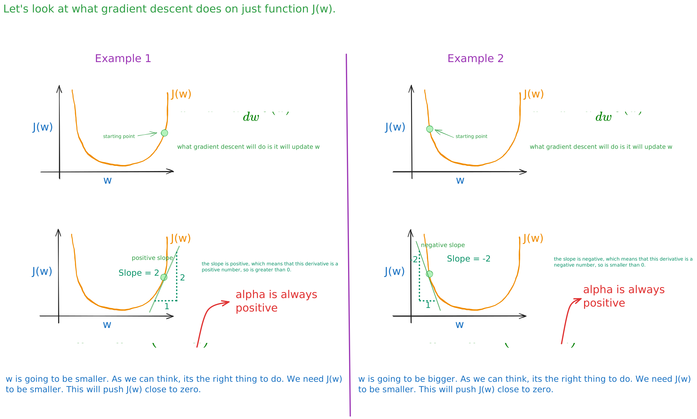
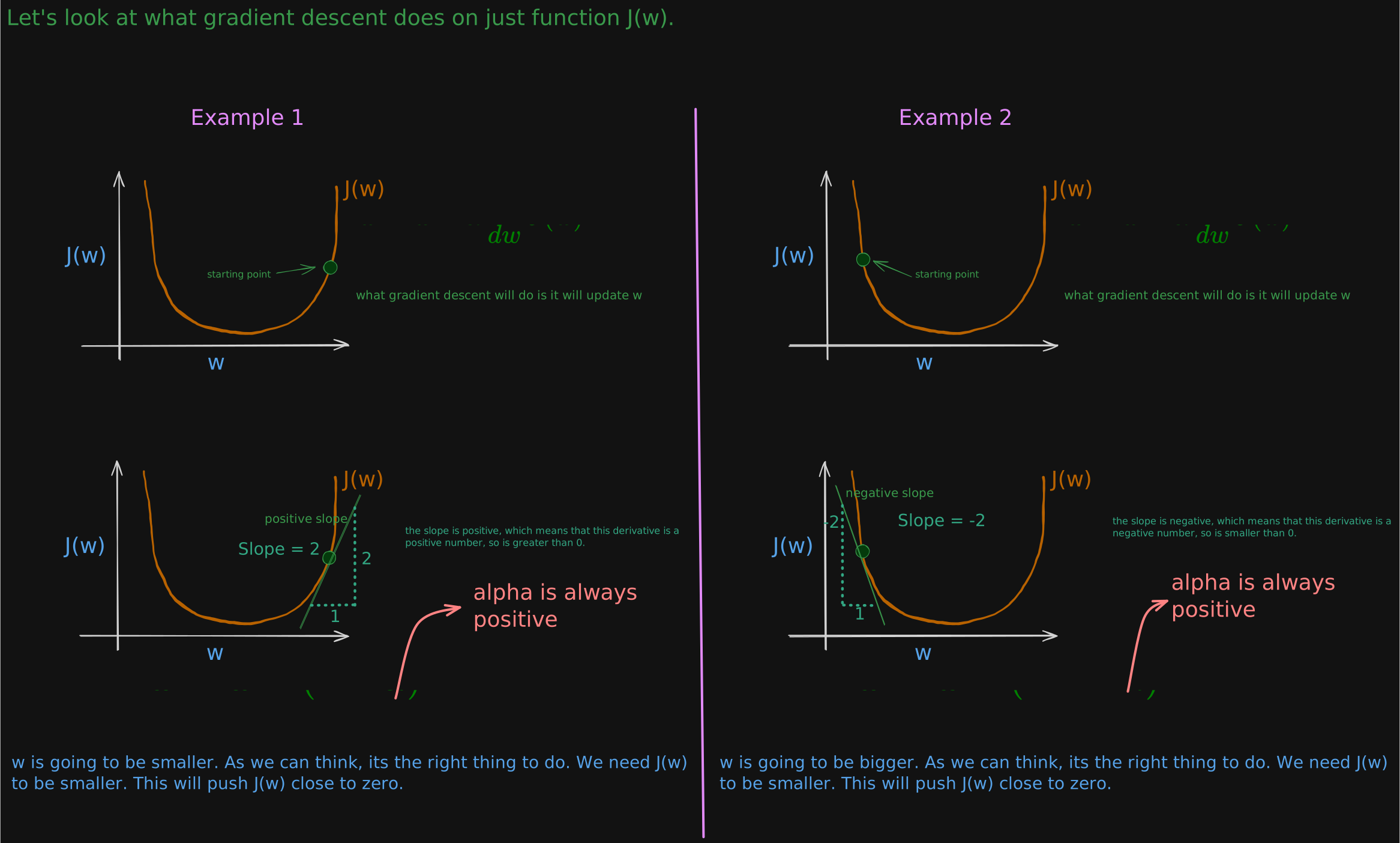
Therefore from two examples, we can say that there are two possibilities here:
Example 1: The updated w is going to be w minus the learning rate times some positive number. The learning rate is always a positive number. If you take w minus a positive number, you end up with a new value for w, that’s smaller. On the graph, you’re moving to the left, you’re decreasing the value of w. You may notice that this is the right thing to do if your goal is to decrease the cost J, because when we move towards the left on this curve, the cost j decreases, and you’re getting closer to the minimum for J, which is over here.
; this will decrease
Example 2: The updated w is going to be w minus the learning rate times some negative number. The learning rate is always a positive number. If you take w minus a negative number, you end up with a new value for w, that’s bigger. On the graph, you’re moving to the right, you’re increasing the value of w. You may notice that this is the right thing to do if your goal is to decrease the cost J, because when we move towards the right on this curve, the cost j decreases, and you’re getting closer to the minimum for J, which is over here.
; this will increase
Learning Rate Intuition
One other key quantity in the gradient descent algorithm is the learning rate Alpha. How do you choose Alpha? What happens if it’s too small or what happens when it’s too big?
The choice of the learning rate, alpha will have a huge impact on the efficiency of your implementation of gradient descent. And if alpha, the learning rate is chosen poorly gradient descent may not even work.
There are three possibility of (learning rate):
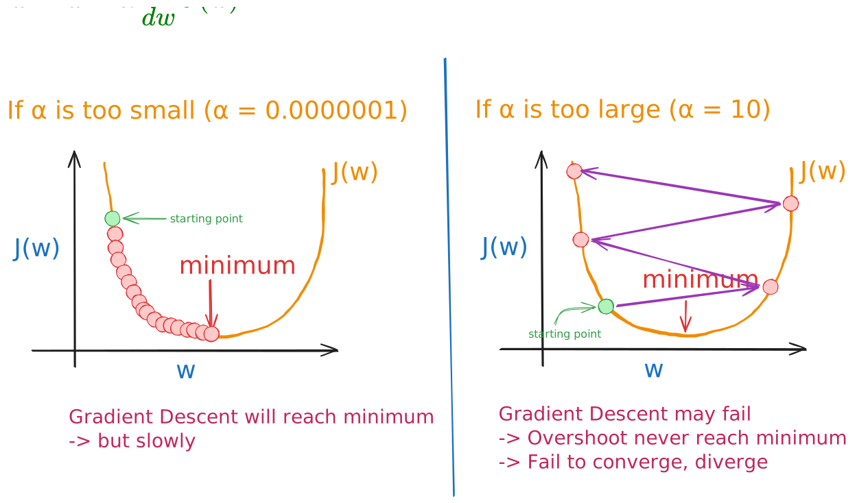
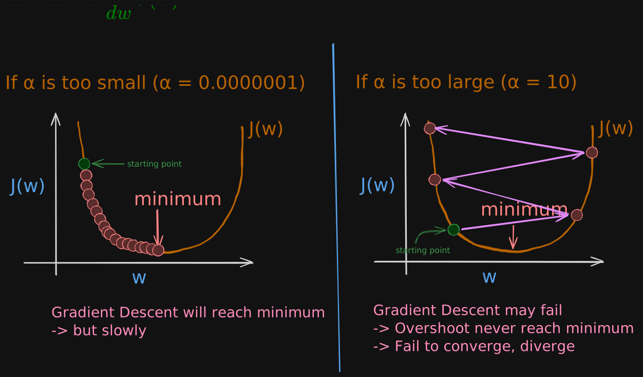
If is too small (surely but slowly):
So to summarize if the learning rate is too small, then gradient descent will work, but it will be slow. It will take a very long time because it’s going to take these tiny tiny baby steps. And it’s going to need a lot of steps before it gets anywhere close to the minimum.
If is too big (may not converge, and even diverge)
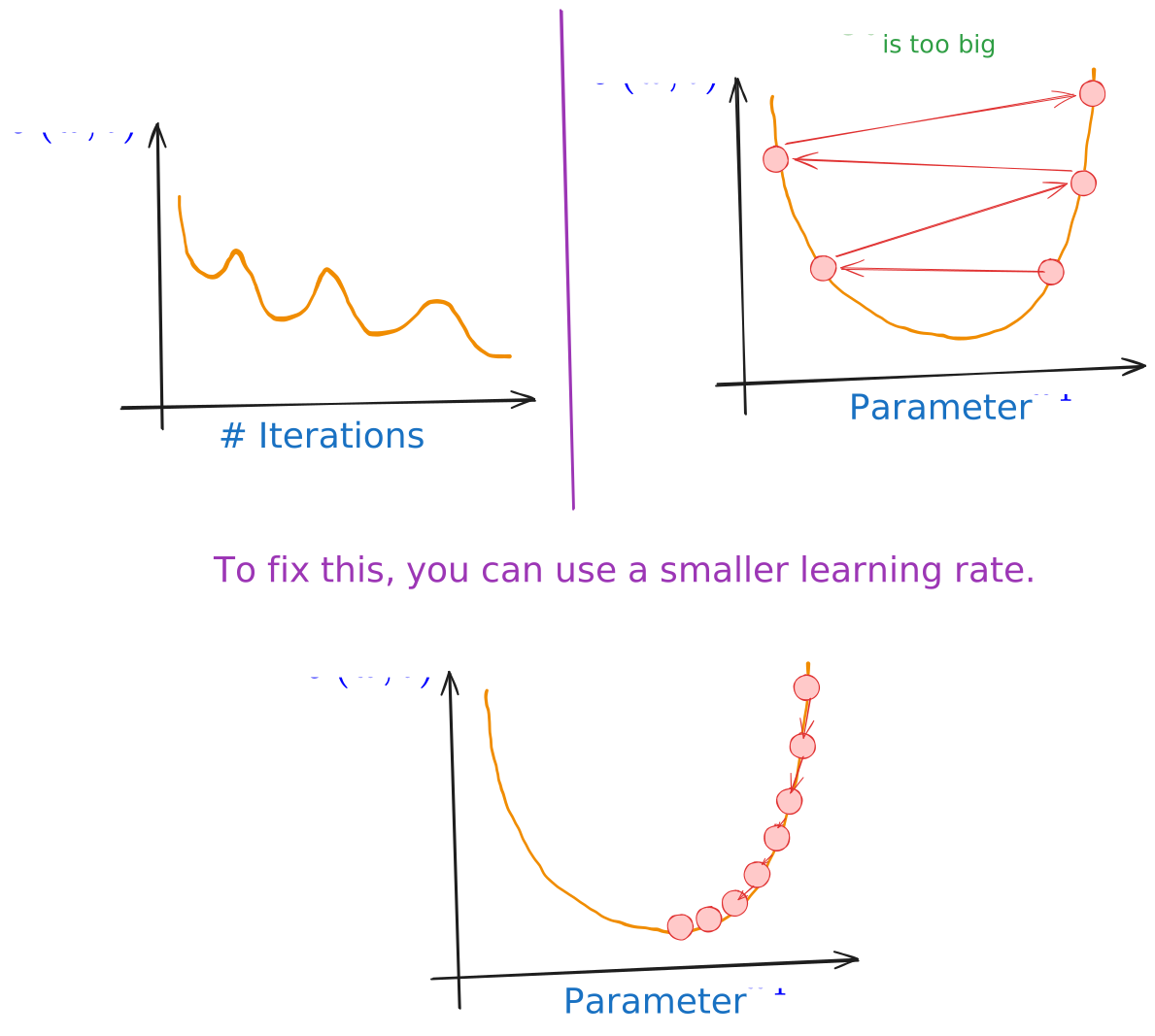
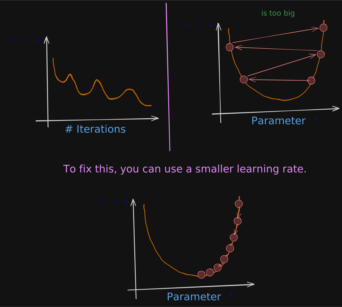
if the learning rate is too large then you take a very large step in w to be all the way over here. And that’s this point here on the . So you move from this point on the left, all the way to this point on the right. And now the cost has actually gotten worse. It has increased because it started out at this value here and after one step, it actually increased to this value here.
Now the derivative at this new point says to decrease w but when the learning rate is too big. Then you may take a huge step going from here all the way out here. So now you’ve gotten to this point here and again, if the learning rate is too big. Then you take another huge step with an acceleration and way overshoot the minimum again. So now you’re at this point on the right and one more time you do another update. And end up all the way here and so you’re now at this point here. So as you may notice you’re actually getting further and further away from the minimum.
So if the learning rate is too large, then gradient descent may overshoot and may never reach the minimum. And another way to say that is that gradient descent may fail to converge and may even diverge.
If is perfect
A perfect is truly a work of art. It’s an active research topic.
Another question, you may be wondering your parameter w is already at this point at local minima. So that your cost J is already at a local minimum. What do you think? One step of gradient descent will do if you’ve already reached a minimum? So this is a tricky one.
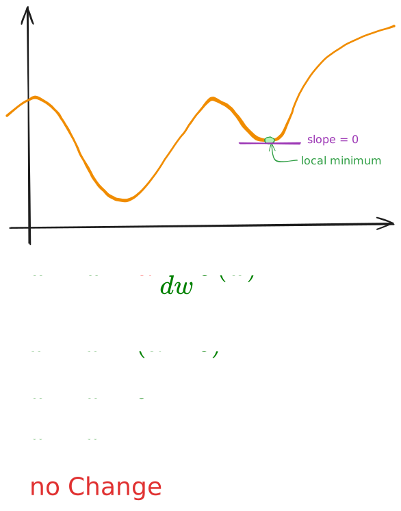
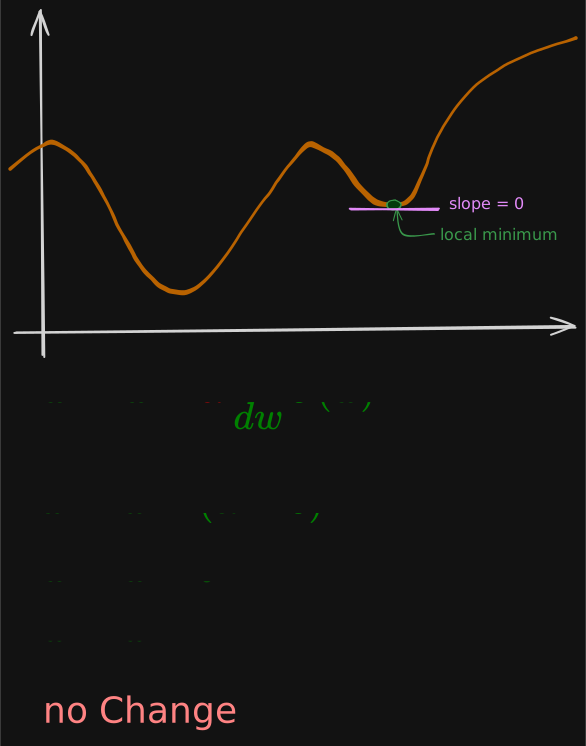
Let’s suppose you have some . And the one you see here isn’t a square error cost function and this cost function has two local minima corresponding to the two valleys that you see here. Now let’s suppose that after some number of steps of gradient descent, your parameter w is over here, say equal to five. And so this is the current value of w. This means that you’re at this point on the . And that happens to be a local minimum, turns out if you draw attention to the function at this point.
The slope of this line is zero and thus the derivative term. Here is equal to zero for the current value of w. And so your gradient descent update becomes w is updated to w minus the learning rate times zero. We’re here that’s because the derivative term is equal to zero. And this is the same as saying let’s set w to be equal to w. So this means that if you’re already at a local minimum, gradient descent leaves w unchanged.
Because it just updates the new value of w to be the exact same old value of w.
So concretely, let’s say if the current value of w is five. And alpha is 0.1 after one iteration, you update w as w minus alpha times zero and it is still equal to five. So if your parameters have already brought you to a local minimum, then further gradient descent steps to absolutely nothing.
It doesn’t change the parameters which is what you want because it keeps the solution at that local minimum.
This also explains why gradient descent can reach a local minimum, even with a fixed learning rate alpha.
Can reach local minimum with fixed learning rate?
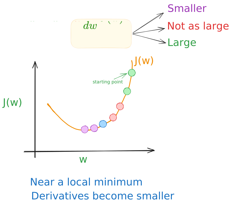
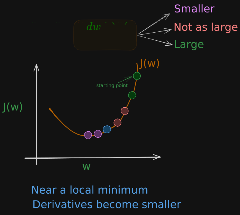
If we take one update step, maybe it will take us to that point. And because this derivative is pretty large, gradient descent takes a relatively big step right. Now, we’re at this second point where we take another step. And you may notice that the slope is not as steep as it was at the first point. So the derivative isn’t as large.
And so the next update step will not be as large as that first step. Now, at this third point here and the derivative is smaller than it was at the previous step. And will take an even smaller step as we approach the minimum. The derivative gets closer and closer to zero. So as we run gradient descent, eventually we’re taking very small steps until you finally reach a local minimum.
So just to recap, as we get nearer a local minimum gradient descent will automatically take smaller steps. And that’s because as we approach the local minimum, the derivative automatically gets smaller.
And that means the update steps also automatically gets smaller. Even if the learning rate alpha is kept at some fixed value.
Gradient Descent for Linear Regression Model
we’re going to pull out together and use the squared error cost function for the linear regression model with gradient descent. This will allow us to train the linear regression model to fit a straight line to achieve the training data.
Linear Regression Model
Cost Function
Gradient Descent Algorithm
If we calculate this derivatives, we get
They’re derived using calculus. Deriving these equations:
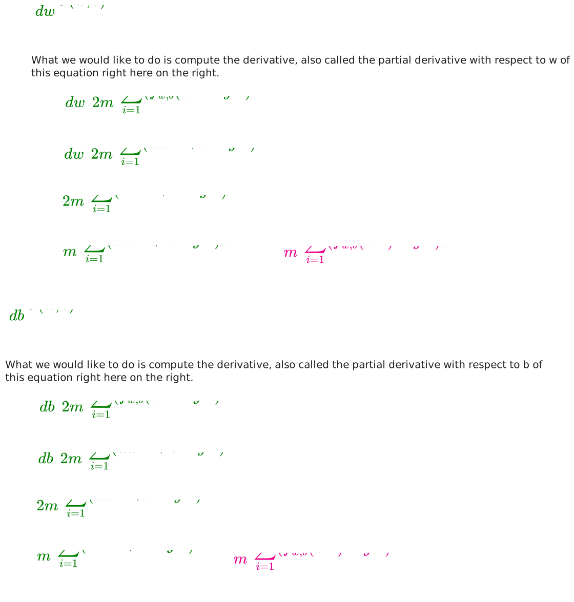
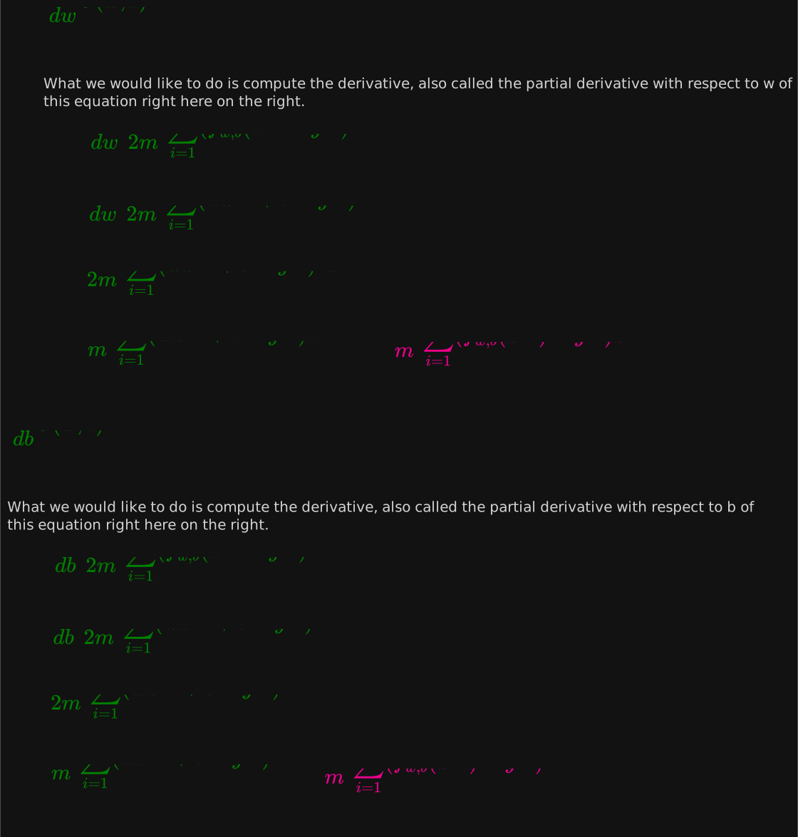
Here’s the gradient descent algorithm for linear regression. You repeatedly carry out these updates to w and b until convergence.
Now, let’s get familiar with how gradient descent works. One issue we saw with gradient descent is that it can lead to a local minimum instead of a global minimum. The global minimum is the point that has the lowest possible value for the cost function J of all possible points.
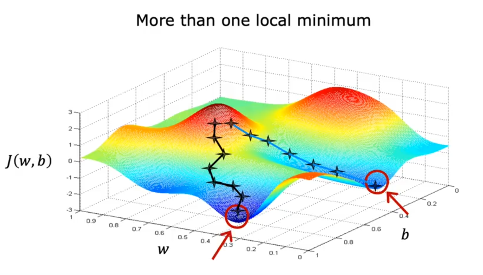
You may recall this surface plot that looks like an outdoor park with a few hills with the process. This function has more than one local minimum. Remember, depending on where you initialize the parameters w and b, you can end up at different local minima. You can end up here, or you can end up here.
But it turns out when you’re using a squared error cost function with linear regression, the cost function does not and will never have multiple local minima. It has a single global minimum because of this bowl-shape. The technical term for this is that this cost function is a convex function.
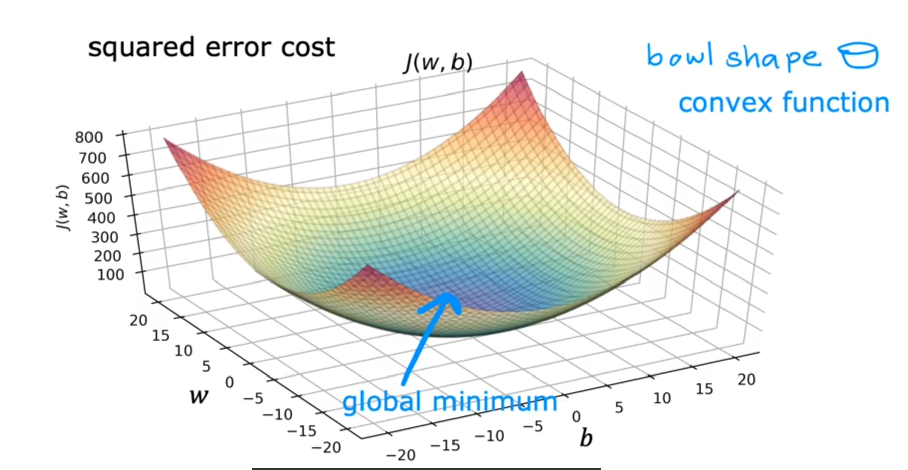
Informally, a convex function is of bowl-shaped function and it cannot have any local minima other than the single global minimum. When you implement gradient descent on a convex function, one nice property is that so long as you’re learning rate is chosen appropriately, it will always converge to the global minimum.
Action
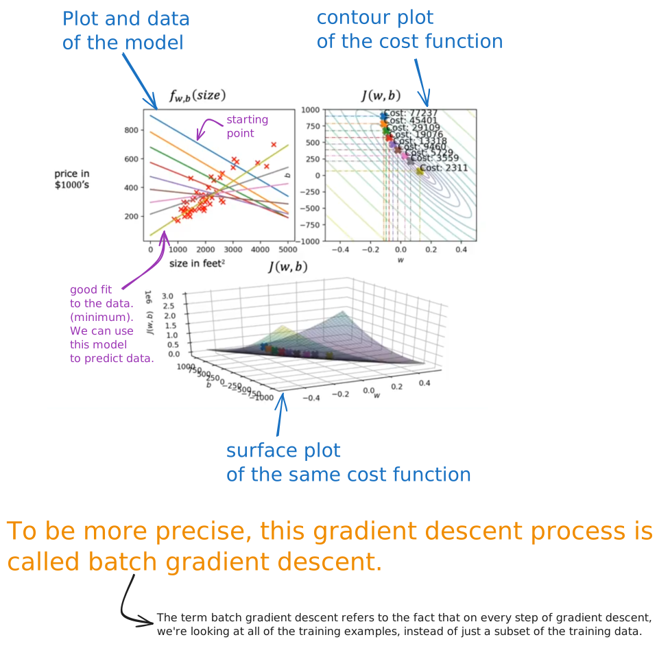
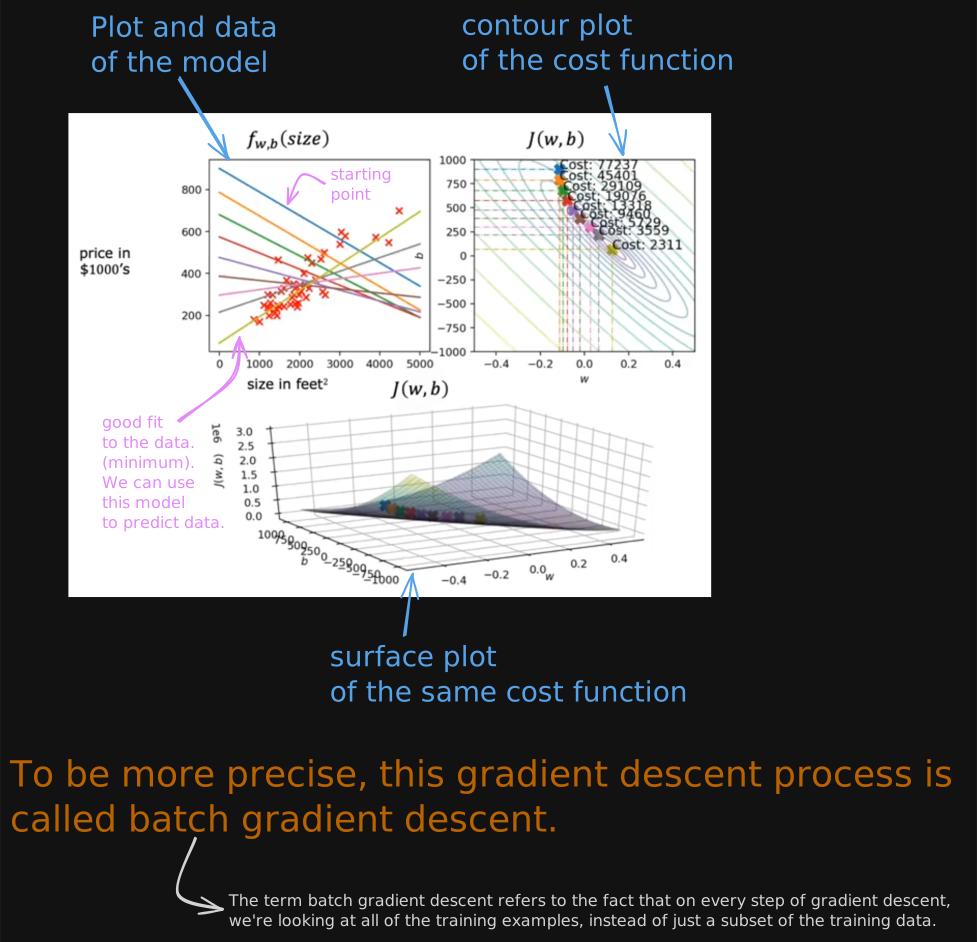
To be more precise, this gradient descent process is called batch gradient descent. The term batch gradient descent refers to the fact that on every step of gradient descent, we’re looking at all of the training examples, instead of just a subset of the training data.
Implementation Code
Look at Lab: Linear Regression with One Feature
Linear Regression Model with Multiple Features
Let’s extend linear regression to handle multiple input features.
Called Multiple Linear Regression! (not multivariate regression - it’s something else)
Multiple Features
In the original version of linear regression, you had a single feature X, the size of the house and you’re able to predict y, the price of the house. But now, what if you did not only have the size of the house as a feature with which to try to predict the price, but if you also knew the number of bedrooms, the number of floors and the age of the home in years.
| Size in () | Number of Bedrooms () | Number of Floors () | Age of home in years () | Price (1000’s (y) |
|---|---|---|---|---|
| 2104 | 5 | 1 | 45 | 460 |
| 1416 | 3 | 2 | 40 | 232 |
| 1532 | 3 | 2 | 30 | 315 |
| 852 | 2 | 1 | 36 | 178 |
| ... | ... | ... | ... | ... |
we’re going to use the variables , , and , to denote the four features.
To refer to specific values, we use two indices: where denotes training example and denotes feature.
For example:
Let’s look at how our model would look like in general with features.
model with n features.
In mathematics, it’s called a vector, which just means a list of numbers.
b is a single number and not a vector.
and are parameters of the model
It is also a vector
Therefore we can rewrite this model as:
What is this dot product thing? Well, the dot products of two vectors of two lists of numbers w and X, is computed by checking the corresponding pairs of numbers, and multiplying that, multiplying that, multiplying that, all the way up to and multiplying that and then summing up all of these products.
The dot product notation lets you write the model in a more compact form with fewer characters.
The name for this type of linear regression model with multiple input features is multiple linear regression. This is in contrast to univariate regression, which has just one feature.
By the way, you might think this algorithm is called multivariate regression, but that term actually refers to something else that we won’t be using here.
In order to implement this, there’s a really neat trick called vectorization, which will make it much simpler to implement this and many other learning algorithms.
Vectorization
vectorization will both make your code shorter and also make it run much more efficiently.
In python and numpy, we can write code like this:
import numpy as np

w = np.array([1.0, 2.5, -3.5])
b = 4
X = np.array([10, 20, 30])
In python, indexing starts at 0. So
Without Vectorization
f = w[0] * X[0] + w[1] * X[1] + w[2] * X[2] + bThe math uses , but Python indexes from 0, so the code uses X[0], X[1], X[2].
what if number of inputs (n) would be 100 or 1000? We can loop it !
In mathematics, we could use summation to add all the products of and
In code
f = 0
for j in range(0, n, 1):
	f = f + w[j] * X[j]

f = f + b
With Vectorization
This is the math expression of the function f,
in Code:
import numpy as np

f = np.dot(w, X) + b
This NumPy dot function is a vectorized implementation of the dot product operation between two vectors and especially when n is large, this will run much faster than the two previous code examples.
What are the benefits?
First, it makes code shorter, is now just one line of code. Isn’t that cool?
Second, it also results in your code running much faster than either of the two previous implementations that did not use vectorization.
The reason that the vectorized implementation is much faster is behind the scenes. The NumPy dot function is able to use parallel hardware in your computer and this is true whether you’re running this on a normal computer, that is on a normal computer CPU or if you are using a GPU, a graphics processor unit, that’s often used to accelerate machine learning jobs. The ability of the NumPy dot function to use parallel hardware makes it much more efficient than the for loop or the sequential calculation that we saw previously.
Also its core part is written in optimized C! and C is fast!, how about we added optimization also! hehe!
Example
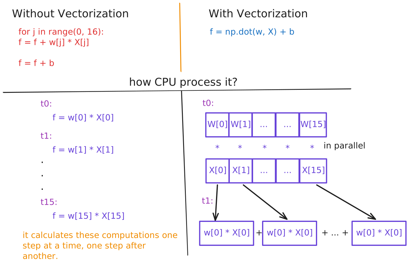
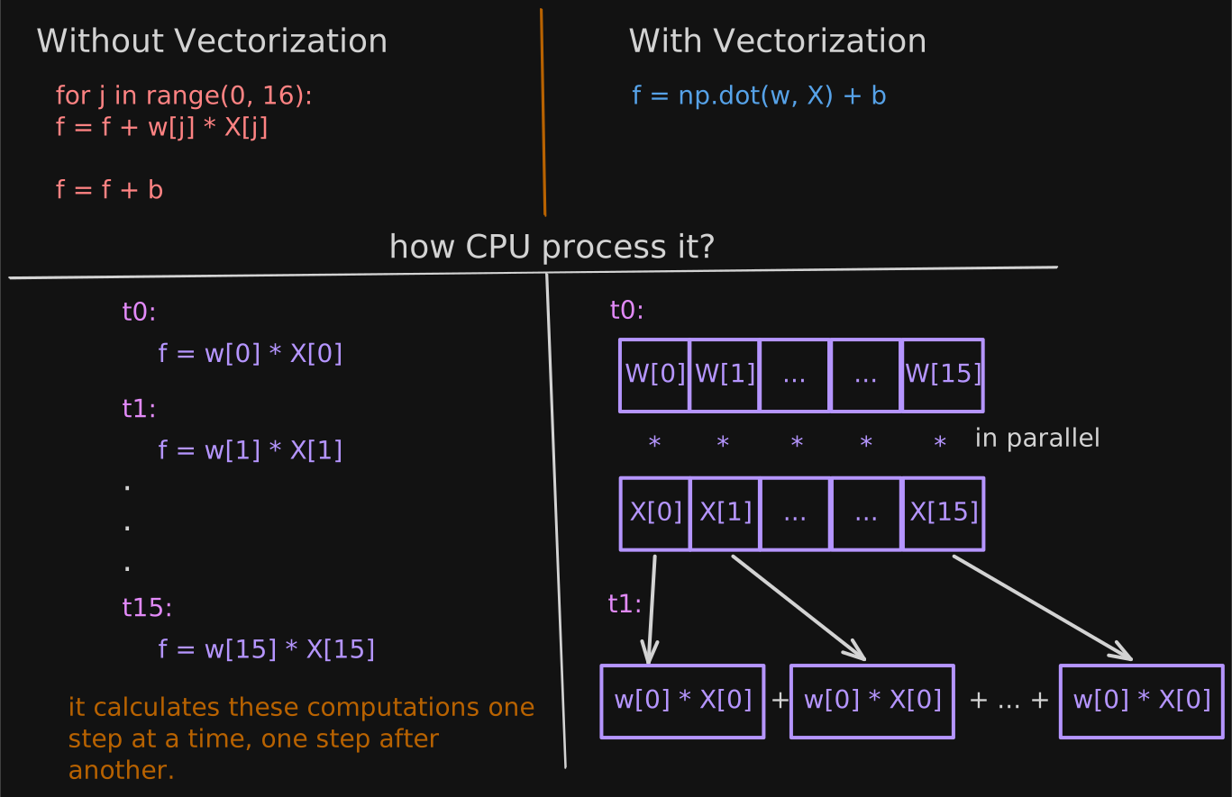
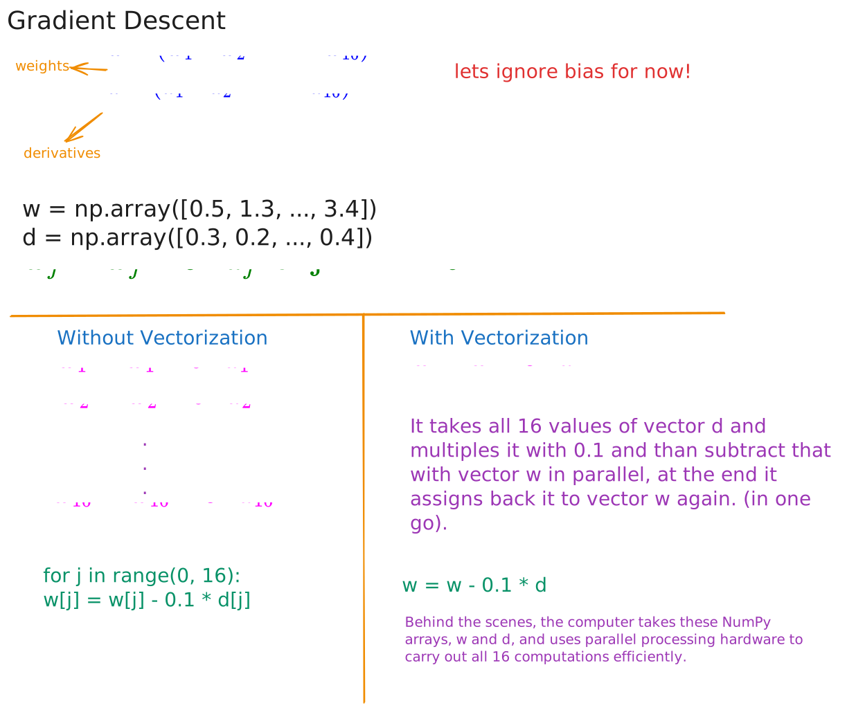
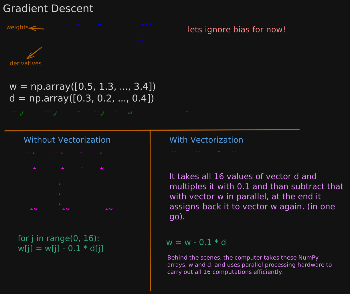
Using a vectorized implementation, you should get a much more efficient implementation of linear regression. Maybe the speed difference won’t be huge if you have 16 features, but if you have thousands of features and perhaps very large training sets, this type of vectorized implementation will make a huge difference in the running time of your learning algorithm. It could be the difference between codes finishing in one or two minutes, versus taking many hours to do the same thing.
To recap, vectorization makes your code shorter, so hopefully easier to write and easier for you or others to read, and it also makes it run much faster.
Gradient Descent for Multiple Linear Regression
| Previous Notation | Vector Notation | |
|---|---|---|
| Parameters | and b | and b is still a number |
| Model | ||
| Cost Function | ||
| Gradient Descent | See (1) below | See (2) below |
(1) Gradient Descent in previous notation:
(2) Gradient Descent in Vector Notation:
Let’s look at how gradient descent works for multiple features
We know that how it works for single feature:
Now, here is the new notation when we have features.
If you implement this, you get gradient descent for multiple regression.
Alternative of Gradient Descent - Normal Equation
There is an alternative way to find and for linear regression, called the normal equation.
the normal equation method, it turns out to be possible to use an advanced linear algebra library to just solve for w and b all in one go without iterations. Though it works only for Linear Regression
Normal Equation:
Only for Linear Regression
Solve for without iterations
Disadvantages?
Doesn’t generalize to other learning algorithms
unlike gradient descent, this is not generalized to other learning algorithms, such as the logistic regression algorithm
Slow when number of features is large (> 10,000)
Feature Scaling
With just a few tricks such as picking and scaling features appropriately and also choosing the learning rate alpha appropriately, you’d really make this work much better.
feature scaling enable gradient descent to run much faster.
Let’s start by taking a look at the relationship between the size of a feature that is how big are the numbers for that feature and the size of its associated parameter.
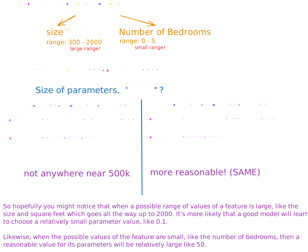
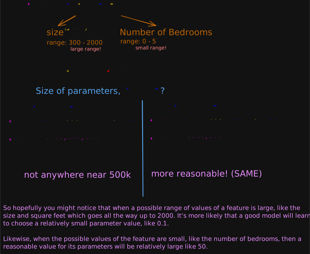
So how does this relate to gradient descent?
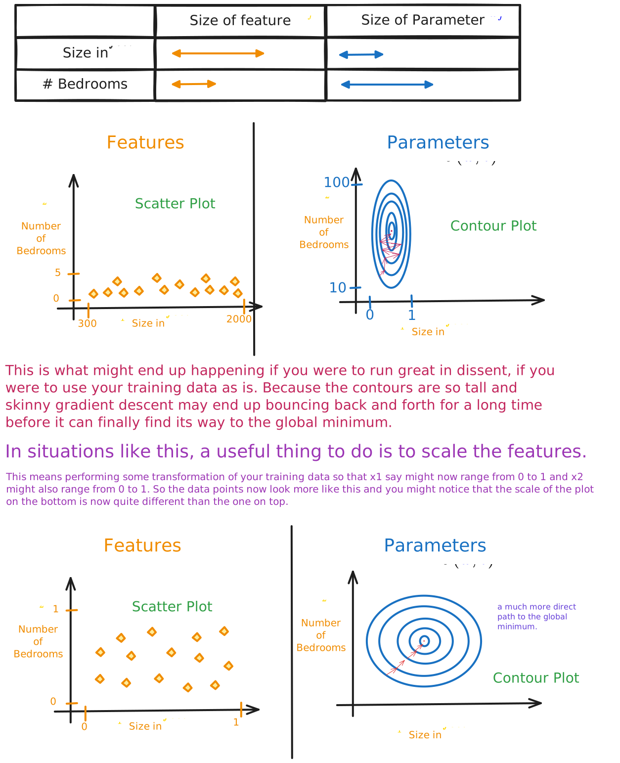
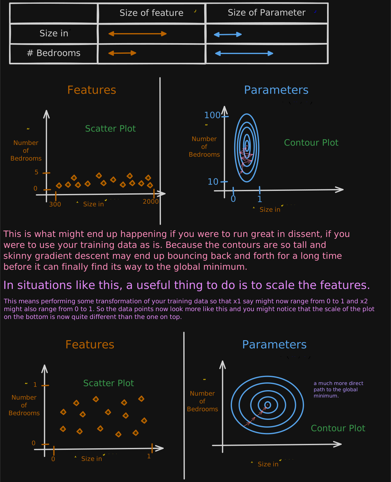
So to recap, when you have different features that take on very different ranges of values, it can cause gradient descent to run slowly but re scaling the different features so they all take on comparable range of values. can speed up gradient descent significantly.
How to do Feature Scaling?
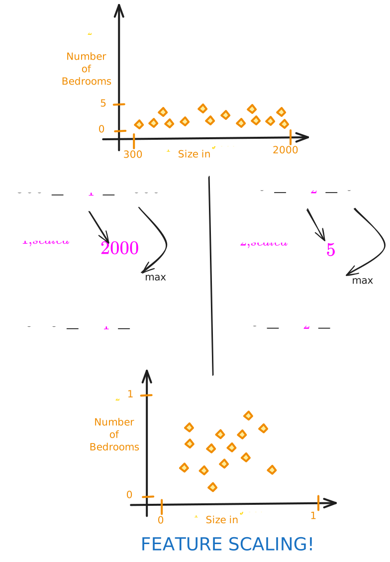
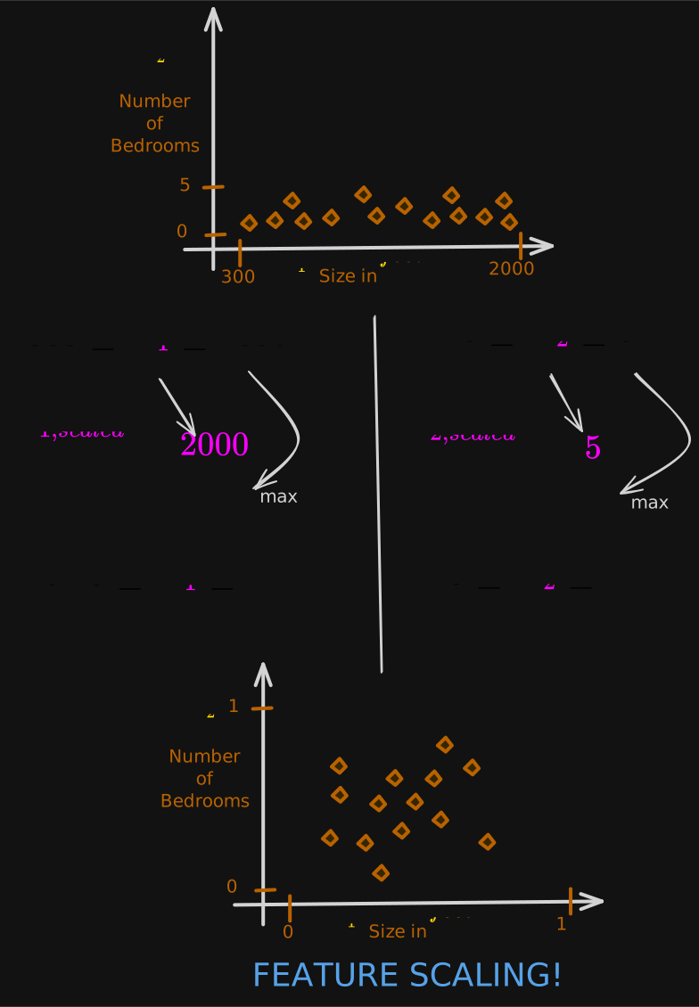
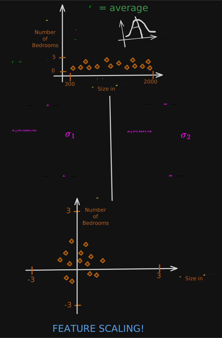
feature scaling is to take features that take on very different ranges of values and scale them to have comparable ranges of values to each other.
Method 1: Divide by Max Value
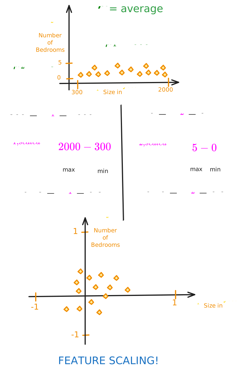
Method 2: Mean Normalization
What this looks like is, you start with the original features and then you re-scale them so that both of them are centered around zero. Whereas before they only had values greater than zero, now they have both negative and positive values that may be usually between negative one and plus one.
To Apply Mean Normalization:
First find the average, also called the mean of , let’s call it
Note:
Apply Feature Scaling:
Method 3: Z-Score Normalization
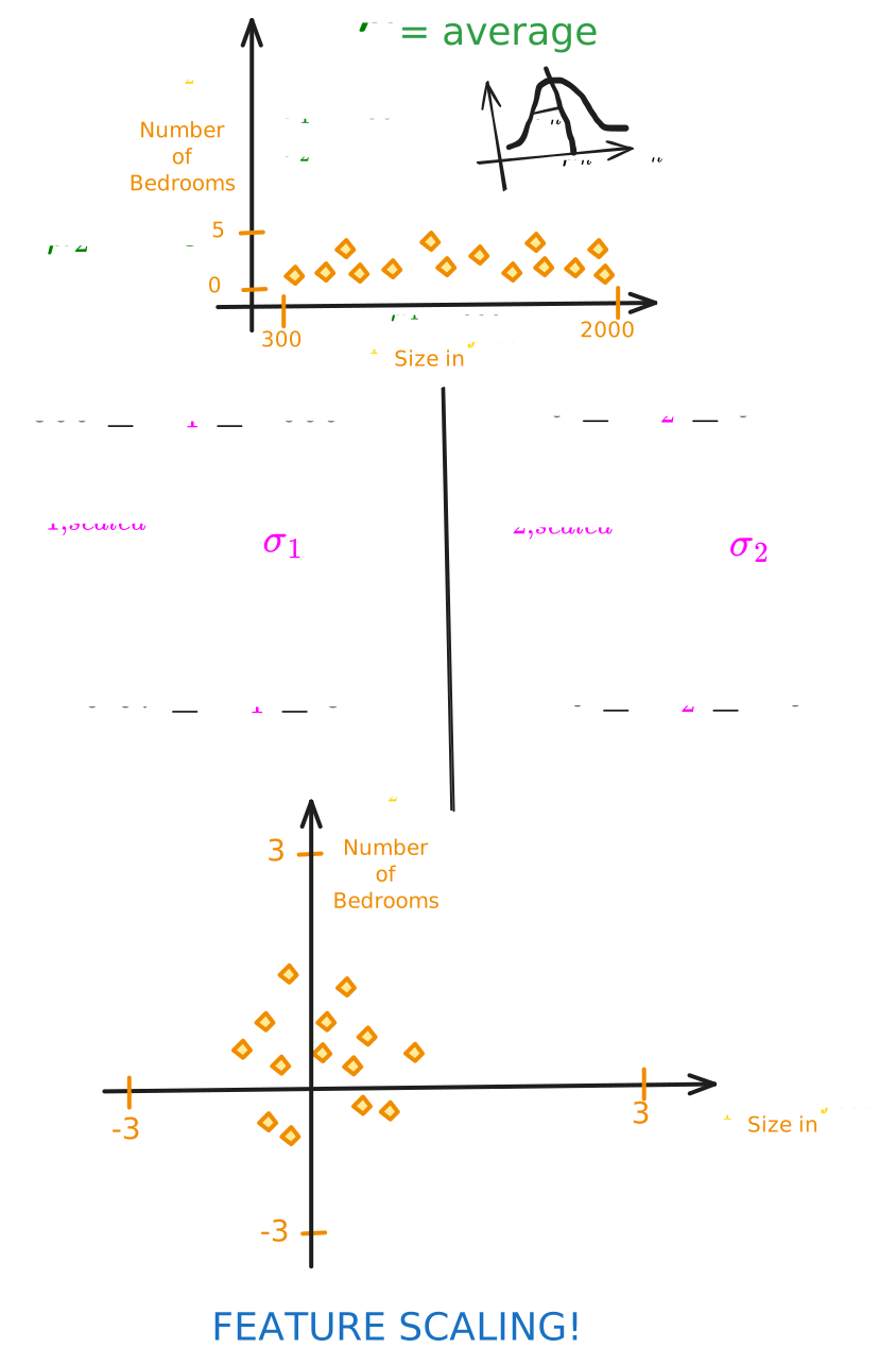
To implement a Z-score normalization,
you first calculate the mean , as well as the standard deviation of each feature.
Apply Feature Scaling:
Thumb Rule
As a rule of thumb, when performing feature scaling, you might want to aim for getting the features to range from maybe anywhere around negative one to somewhere around plus one for each feature X.
aim for about for each feature But these values, negative one and plus one can be a little bit loose.
For Example, if the features ranges from:
All of these are completely acceptable.
If you have a feature:
You can re-scale it if you want, but if you don’t re-scale it, it should work okay too. (No harm)
But if you have feature:
--> Too Large
--> Too Small You’re probably better off re-scaling this feature so that it ranges from something closer to -1 to +1.
Finally, what if your feature , such as measurements of a hospital patients by the temperature ranges from 98.6-105 degrees Fahrenheit?
In this case, these values are around 100, which is actually pretty large compared to other scale features, and this will actually cause gradient descent to run more slowly. In this case, feature re-scaling will likely help.
There’s almost never any harm to carrying out feature re-scaling. When in doubt, I encourage you to just carry it out.
That’s it for feature scaling! With this little technique, you’ll often be able to get gradient descent to run much faster.
Is Gradient Descent Converging?
With or without feature scaling, when you run gradient descent, how can you know, how can you check if gradient descent is really working? If it is finding you the global minimum or something close to it. let’s take a look at how to recognize if gradient descent is converging!
When running gradient descent, how can you tell if it is converging? That is, whether it’s helping you to find parameters close to the global minimum of the cost function.
Objective of Gradient Descent:
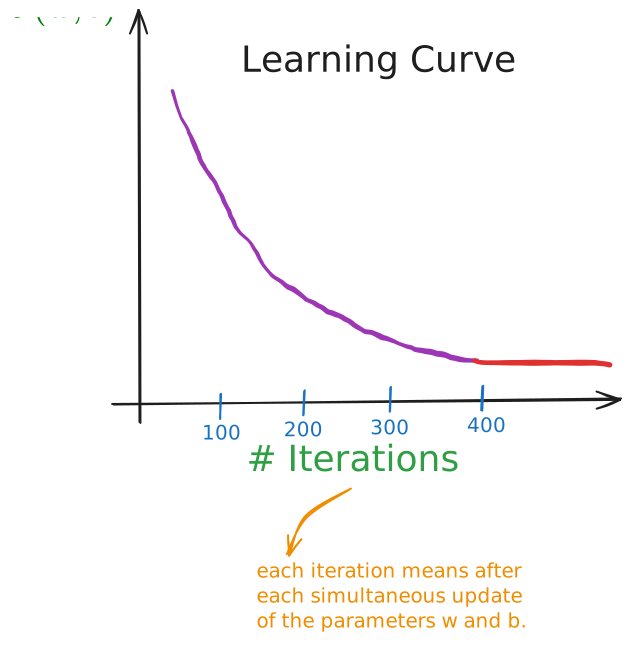
If gradient descent is working properly, then the cost J should decrease after every single iteration.
If J ever increases after one iteration, that means either is chosen poorly, and it usually means is too large, or there could be a bug in the code.
Another useful thing that this plot can tell you is that if you look at this curve, by the time you reach maybe 300 iterations also, the cost J is leveling off and is no longer decreasing much. After 400 iterations, it looks like the curve has flattened out. This means that gradient descent has more or less converged because the curve is no longer decreasing.
Looking at this learning curve, you can try to spot whether or not gradient descent is converging. By the way, the number of iterations that gradient descent takes to converge can vary a lot between different applications. In one application, it may converge after just 30 iterations. For a different application, it could take 1,000 or 100,000 iterations. It turns out to be very difficult to tell in advance how many iterations gradient descent needs to converge, which is why you can create a graph like this, a learning curve.
Ways to find out model is done training?
you can create a graph of learning curve.
Another way to decide when your model is done training is with an automatic convergence test.
Automatic Convergence Test
Let “epsilon” be 10-3 (or 0.001)
If the cost decreases by in one iteration, declare convergence.
In practice, choosing the right threshold is difficult.
In practice, looking at the learning curve is usually more reliable than relying on an automatic convergence test.
Choosing the Learning Rate
Your learning algorithm will run much better with an appropriate choice of learning rate. If it’s too small, it will run very slowly and if it is too large, it may not even converge.
Concretely, if you plot the cost for a number of iterations and notice that the costs sometimes goes up and sometimes goes down, you should take that as a clear sign that gradient descent is not working properly.
This could mean that there’s a bug in the code.
Or sometimes it could mean that your learning rate is too large.
A Common Bug: Wrong Sign
In code you may be doing:
but you should use minus sign
This is because having the derivative term moves your cost J further from the global minimum instead of closer.
Feature Engineering
The choice of features can have a huge impact on your learning algorithm’s performance. In fact, for many practical applications, choosing or engineering the right features is a critical step to making the algorithm work well.
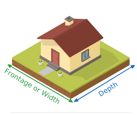
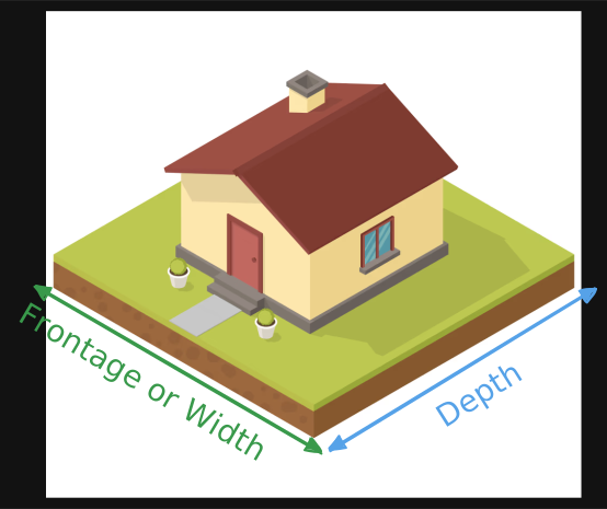
Let’s say:
is the width of the lot size of the plots of land that the house is built on. This in real estate is also called the frontage of the lot
is the depth of the lot size.
Model : This model might work okay.
But here’s another option for how you might choose a different way to use these features in the model that could be even more effective. You might notice that the area of the land can be calculated as the frontage or width times the depth.
You may have an intuition that the area of the land is more predictive of the price, than the frontage and depth as separate features.
New Model:
What we just did, creating a new feature is an example of what’s called feature engineering, in which you might use your knowledge or intuition about the problem to design new features usually by transforming or combining the original features of the problem in order to make it easier for the learning algorithm to make accurate predictions.
Full Implementation
Look at Lab: Linear Regression with Multiple Feature
Summary
Linear Regression is probably the single most widely used learning algorithm in the world today.
Solution to Exercise 3.2
False - Doubling the learning rate may result in a learning rate that is too large, and cause gradient descent to fail to find the optimal values for the parameters w, and b.
- Ng, Dr. A. (2022). Machine Learning Specialization. Coursera. https://www.coursera.org/specializations/machine-learning-introduction