Lab: Linear Regression with multiple feature

While not max_steps:
    1.Find J(w, b)
    2.Find new Weight, and Bias using Gradient Descent

    if new J(w, b) and old J(w, b) has no or very less different
        break

import numpy as np

class LinearRegression:
    def __init__(self, n_iter=10000, convergence_limit=1e-7, learning_rate=0.01):
        self.n_iter = n_iter
        self.convergence_limit = convergence_limit
        self.learning_rate = learning_rate

    def _model(self, X):
        y_hat = np.dot(X, self.weights) + self.bias

        return y_hat

    def _cost_function(self):
        f_wb = self._model(self.X)
        
        J_wb = f_wb - self.y
        J_wb = J_wb ** 2
        J_wb = np.sum(J_wb)
        J_wb = J_wb / (2 * self.m)    

        return J_wb

    def _gradient(self):
        dL_dw = np.zeros(self.n)
        dL_db = 0

        for i in range(self.m):
            dL_df = self._model(self.X[i]) - self.y[i]

            dL_dw += dL_df * self.X[i]
            dL_db += dL_df

        dL_dw = dL_dw / self.m
        dL_db = dL_db / self.m

        return dL_dw, dL_db

    def _gradient_descent(self):
        for i in range(self.n_iter):
            dL_dw, dL_db = self._gradient()

            w_temp = self.weights - self.learning_rate * dL_dw
            b_temp = self.bias - self.learning_rate * dL_db

            self.weights = w_temp
            self.bias = b_temp

            self.history.append(self._cost_function())
            
            converged = len(self.history) > 1 and abs(self.history[-1] - self.history[-2]) < self.convergence_limit
            diverged = not np.isfinite(self.history[-1])
            
            if converged or diverged:
                break

        return self
      
    def fit(self, X, y):
        X = np.asarray(X, dtype=float)
        y = np.asarray(y, dtype=float)

        if X.ndim == 1:
            X = X.reshape(-1, 1)

        # Feature Scaling "z-score"
        self.mean = np.mean(X, axis=0)

        self.std = np.std(X, axis=0)
        self.std[self.std == 0] = 1.0


        self.X = (X - self.mean) / self.std
        self.y = y

        self.m = self.X.shape[0] # Number of Data Rows
        self.n = self.X.shape[1] # Number of Features

        self.weights = np.zeros(self.n)
        self.bias = 0

        self.history = []

        # Finding best parameters
        self._gradient_descent()

        return self

    def predict(self, X):
        X = np.asarray(X, dtype=float)
        # Feature Rescaling (for test data)
        X = (X - self.mean) / self.std
        
        y_hat = self._model(X)

        print("mean:", self.mean, "std:", self.std)
        print("Weights:", self.weights)
        print("Bias:", self.bias)
        print("Prediction:", y_hat)

# Test Data
# y = 4.5*x1 - 2.8*x2 + 3.2 + noise (noise std = 4), 100 samples

X = np.array([
    [  2.74,  -0.61],
    [  3.59,   1.97],
    [ -4.06,   4.76],
    [  2.61,   2.86],
    [ -3.72,  -0.50],
    [ -1.29,   4.27],
    [  1.44,   3.23],
    [ -0.57,  -2.73],
    [  0.55,  -4.36],
    [  3.28,   1.32],
    [  2.58,  -1.45],
    [  4.71,   3.93],
    [  2.78,  -3.05],
    [ -0.33,  -4.56],
    [ -3.46,   1.83],
    [  2.45,   4.68],
    [ -1.74,  -1.30],
    [ -0.30,  -3.11],
    [ -3.70,  -0.24],
    [ -2.73,   1.70],
    [ -0.63,   3.33],
    [  2.00,  -1.88],
    [  3.32,   3.05],
    [ -1.13,  -2.12],
    [  1.82,  -3.60],
    [ -3.00,  -4.93],
    [  2.87,   1.65],
    [  2.05,   2.81],
    [ -0.41,   0.69],
    [ -3.60,  -3.85],
    [  1.68,  -0.29],
    [  0.65,   2.65],
    [  1.35,   0.54],
    [  0.59,  -1.96],
    [ -4.69,  -0.63],
    [ -2.85,  -0.91],
    [  3.53,  -2.66],
    [ -4.42,  -2.19],
    [ -2.06,   1.62],
    [  0.57,   2.84],
    [  1.64,  -0.94],
    [  3.14,  -3.33],
    [ -4.77,  -4.10],
    [  2.22,  -0.38],
    [ -3.39,   0.01],
    [ -3.48,   1.96],
    [ -0.54,  -1.19],
    [ -1.98,   1.30],
    [ -1.38,  -4.12],
    [ -3.82,   4.62],
    [  4.09,   2.00],
    [ -2.34,   4.69],
    [  2.79,   2.17],
    [ -0.51,  -2.28],
    [ -4.04,   4.03],
    [ -0.44,  -2.98],
    [ -1.94,   0.79],
    [ -3.23,   3.57],
    [  2.59,   2.19],
    [ -0.68,   1.27],
    [  0.84,   1.50],
    [ -4.16,  -0.84],
    [ -4.58,  -0.06],
    [ -1.70,  -3.55],
    [ -3.97,   0.88],
    [ -3.29,   4.25],
    [  0.81,  -1.53],
    [  0.91,  -4.77],
    [  4.59,  -0.18],
    [  2.83,  -4.17],
    [ -0.13,  -0.09],
    [  4.38,   0.72],
    [ -0.27,  -2.33],
    [ -1.68,   0.21],
    [ -0.61,  -4.78],
    [  3.26,   3.96],
    [ -3.60,   0.54],
    [ -3.91,   1.72],
    [ -2.19,   1.59],
    [  2.27,   2.69],
    [ -3.92,   4.16],
    [ -2.70,  -4.63],
    [  0.55,  -1.29],
    [  3.30,   3.08],
    [ -1.83,   4.53],
    [ -2.09,   0.15],
    [ -2.44,   4.36],
    [ -3.35,  -4.55],
    [ -0.65,   4.92],
    [  3.92,   2.49],
    [  3.91,   3.93],
    [  0.19,  -1.84],
    [  2.72,   1.62],
    [ -1.26,  -4.06],
    [  2.47,  -2.38],
    [  4.37,  -2.59],
    [ -3.77,   3.31],
    [ -3.47,  -3.21],
    [  0.99,   3.75],
    [ -3.04,  -1.90],
])

y = np.array([
      19.81,   12.26,  -28.42,    6.28,  -10.79,
      -8.93,    1.00,   10.85,    9.68,   14.07,
      15.50,    8.52,   20.74,   13.15,  -13.83,
      -4.18,   -0.87,    8.62,  -14.09,   -9.83,
      -6.81,   22.81,    8.98,    1.27,   20.57,
       4.47,   12.20,    0.22,   -0.22,   -1.31,
      21.64,    6.21,    4.35,   10.19,  -21.99,
      -9.44,   27.80,   -5.73,  -13.52,   -4.80,
       4.62,   26.00,  -11.03,   12.14,  -15.59,
     -18.33,   -2.93,  -15.22,   17.04,  -32.08,
      11.62,  -13.11,   21.30,    2.60,  -27.74,
      10.93,   -0.83,  -25.28,    7.74,   -0.31,
       4.52,  -14.67,  -17.78,   -0.01,  -18.08,
     -24.57,   12.06,   18.43,   26.25,   31.66,
       3.49,   22.30,    8.72,   -4.95,   10.95,
       8.05,  -14.90,  -10.84,   -4.81,    7.43,
     -29.14,   -0.44,   14.05,   10.48,  -15.80,
     -13.60,  -16.28,    2.68,  -17.94,   11.98,
      10.85,    9.42,    9.74,    8.48,   19.97,
      30.73,  -17.15,  -13.69,   -3.79,   -4.45,
])

import matplotlib.pyplot as plt

# Extract features
x1 = X[:, 0]
x2 = X[:, 1]

# Create 3D plot
fig = plt.figure(figsize=(10, 7))
ax = fig.add_subplot(111, projection="3d")

# Plot data points
ax.scatter(x1, x2, y, color="blue", s=60, label="Data points")

# Labels
ax.set_xlabel("x1")
ax.set_ylabel("x2")
ax.set_zlabel("y")
ax.set_title("Linear Regression Dataset (2 Features)")

ax.legend()
plt.show()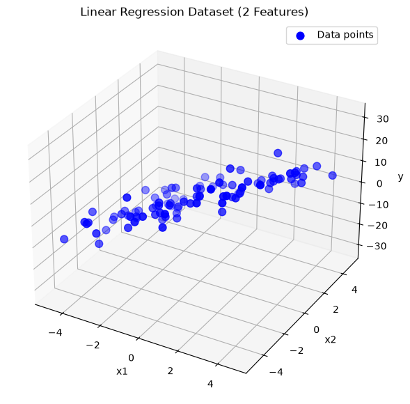

# Four different Linear Regression mode with learning rate change
lr1 = LinearRegression(n_iter=10000, convergence_limit=1e-7, learning_rate=0.01)
lr2 = LinearRegression(n_iter=10000, convergence_limit=1e-7, learning_rate=0.001)
lr3 = LinearRegression(n_iter=10000, convergence_limit=1e-7, learning_rate=0.0001)
lr4 = LinearRegression(n_iter=10000, convergence_limit=1e-7, learning_rate=0)

lr1.fit(X, y)
lr2.fit(X, y)
lr3.fit(X, y)
lr4.fit(X, y)

<__main__.LinearRegression at 0x2202f6ee150>

# Predictions --> 3.8

print("LR1")
lr1.predict([2.0, 3.0])

print("LR2")
lr2.predict([2.0, 3.0])

print("LR3")
lr3.predict([2.0, 3.0])

print("LR4")
lr4.predict([2.0, 3.0])

LR1
mean: [-0.299   0.1769] std: [2.7437294 2.8673457]
Weights: [12.40141217 -7.51510148]
Bias: 1.1730256436710773
Prediction: 4.165163846319295
LR2
mean: [-0.299   0.1769] std: [2.7437294 2.8673457]
Weights: [12.39573878 -7.5106585 ]
Bias: 1.1726056602733947
Prediction: 4.16436449310532
LR3
mean: [-0.299   0.1769] std: [2.7437294 2.8673457]
Weights: [ 7.6980177  -4.52180807]
Bias: 0.7416254203248862
Prediction: 2.739843669937235
LR4
mean: [-0.299   0.1769] std: [2.7437294 2.8673457]
Weights: [0. 0.]
Bias: 0.0
Prediction: 0.0

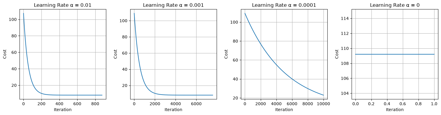
# Cost Function - Loss every iteration
import matplotlib.pyplot as plt

histories = [lr1.history, lr2.history, lr3.history, lr4.history]
alphas = [0.01, 0.001, 0.0001, 0]

fig, axes = plt.subplots(1, 4, figsize=(15, 4))

for i, (history, alpha) in enumerate(zip(histories, alphas)):
    axes[i].plot(history)
    axes[i].set_title(f"Learning Rate α = {alpha}")
    axes[i].set_xlabel("Iteration")
    axes[i].set_ylabel("Cost")
    axes[i].grid(True)

plt.tight_layout()
plt.show()