Chapter 6: Fit The Data Well - AI from First Principles

Sometimes in an application, the algorithm can run into a problem called overfitting, which can cause it to perform poorly. Let’s look at overfitting and its opposite, underfitting.

Technically we say that you want your learning algorithm to generalize well, which means to make good predictions even on brand new examples that it has never seen before.

You can say that the goal of machine learning is to find a model that hopefully is neither underfitting nor overfitting. In other words, hopefully, a model that has neither high bias nor high variance.

Overfitting vs Underfitting¶

Linear Regression¶

Let’s go back to our original example of predicting housing prices with linear regression, where you want to predict the price as a function of the size of a house.

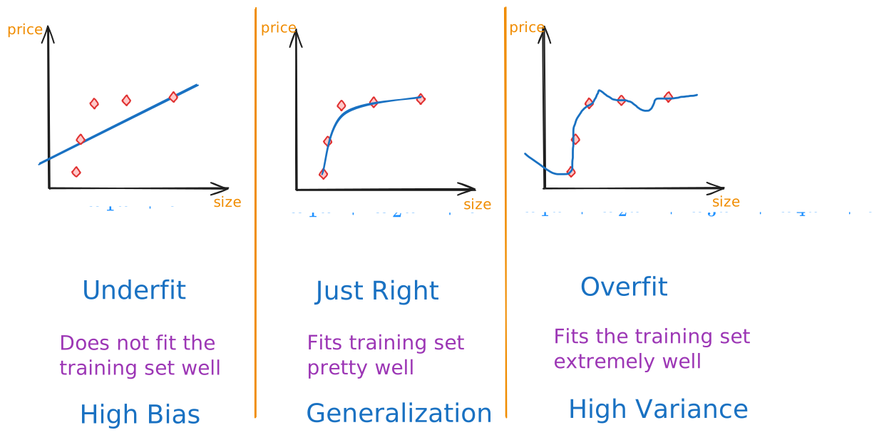
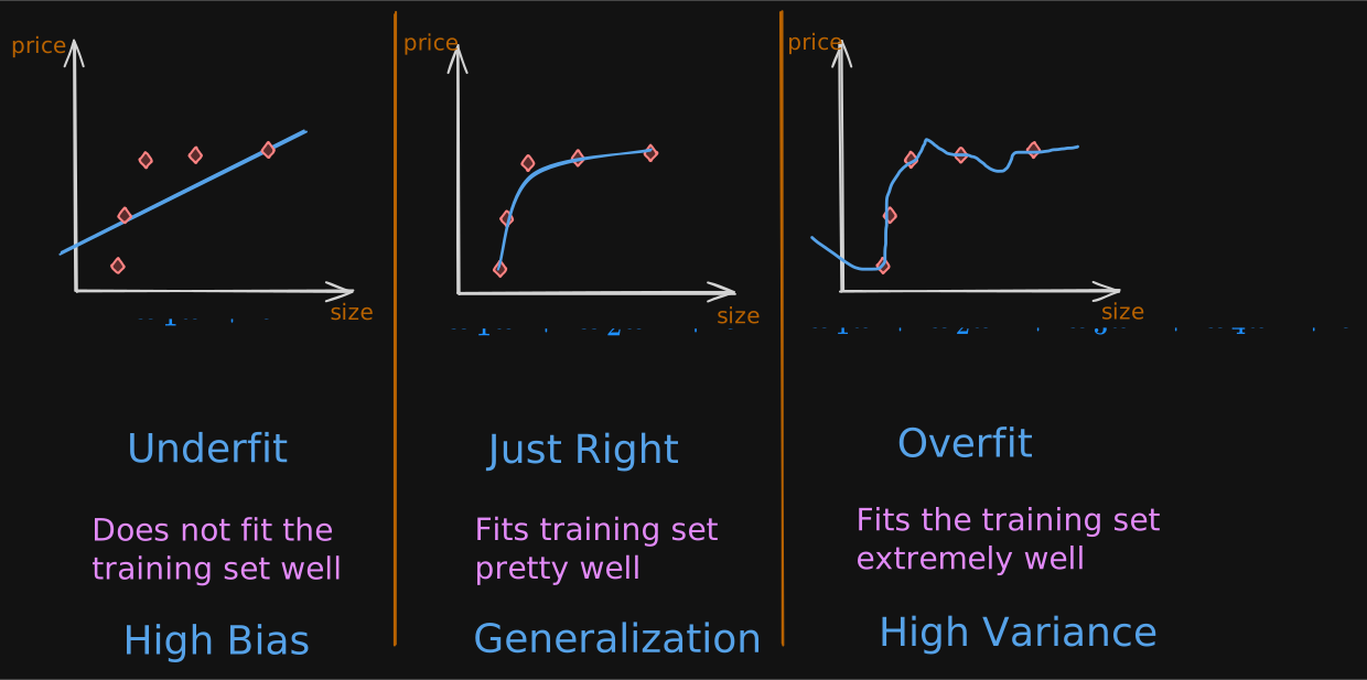
High Variance: If two different machine learning engineers were to fit this fourth-order polynomial model to just slightly different datasets, they could end up with totally different predictions or highly variable predictions. That’s why we say the algorithm has high variance.

STORY: When I think about underfitting and overfitting, high bias and high variance, I’m sometimes reminded of the children’s story of Goldilocks and the Three Bears. In this tale, a girl called Goldilocks visits the home of a bear family. There’s a bowl of porridge that’s too cold to taste and so that’s no good. There’s also a bowl of porridge that’s too hot to eat. That’s no good either. But there’s a bowl of porridge that is neither too cold nor too hot. The temperature is in the middle, which is just right to eat.

Logistic Regression¶

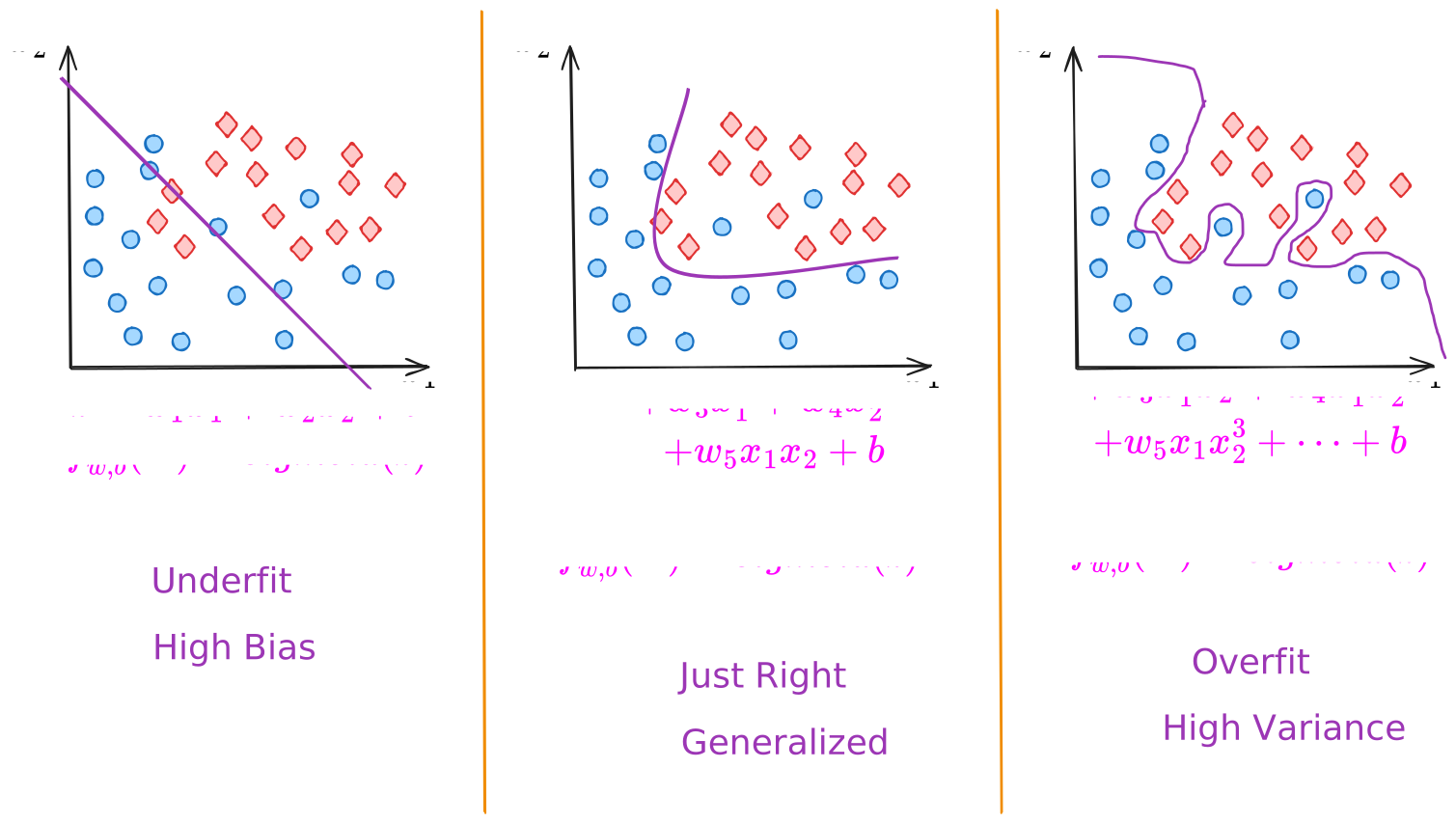
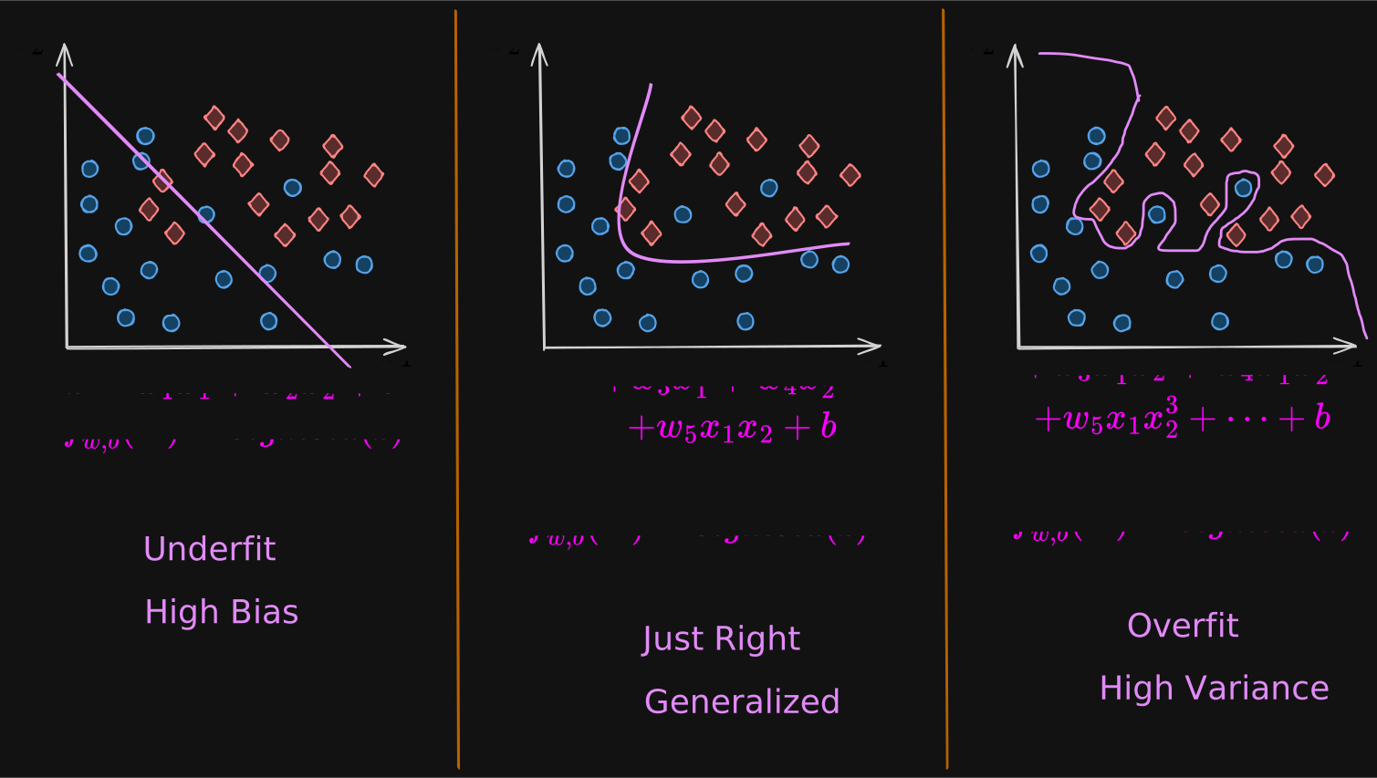
Having all these higher-order polynomial features allows the algorithm to choose this overly complex decision boundary

Now you’ve seen how an algorithm can underfit or have high bias or overfit and have high variance.

Addressing Overfitting¶

When you think overfitting has occurred, let’s talk about what you can do to address it. Let’s say you fit a model and it has high variance, is overfit.

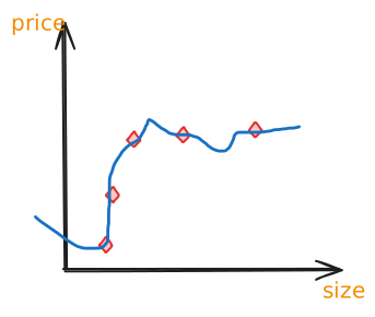
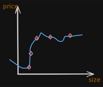
Method 1: Collect more training data¶

If you’re able to get more data, that is more training examples on sizes and prices of houses, then with the larger training set, the learning algorithm will learn to fit a function that is less wiggly.

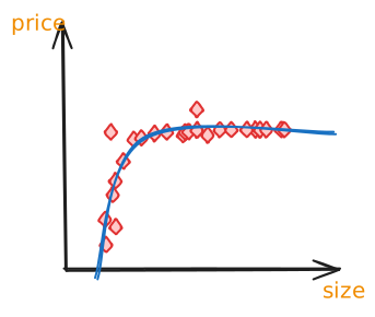
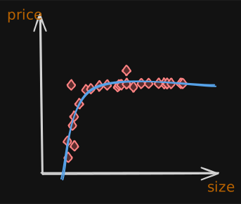
You can continue to fit a high-order polynomial or some other function with a lot of features, and if you have enough training examples, it will still do okay.
To summarize, the number one tool you can use against overfitting is to get more training data.

Method 2: Feature Selection¶

Select features to include/exclude
A second option for addressing overfitting is to see if you can use fewer features.
- For example: $f(x) = w_1 x_1 + w_2 x_2^2 + w_3 x_3^3 + w_4 x_4 ^ 4 + b$
These were a lot of polynomial features. In that case, one way to reduce overfitting is to just not use so many of these polynomial features.
Maybe you have a lot of different features of a house of which to try to predict its price, ranging from the size, number of bedrooms, number of floors, the age, average income of the neighborhood, and so on and so forth, total distance to the nearest coffee shop.
- It turns out that if you have a lot of features like these but don’t have enough training data, then your learning algorithm may also overfit to your training set.
Now instead of using all 100 features, we could pick just a subset of the most useful ones: maybe size, bedrooms, and the age of the house.
- If you think those are the most relevant features, then using just that smallest subset of features, you may find that your model no longer overfits as badly.

Choosing the most appropriate set of features to use is sometimes also called feature selection. One way you could do so is to use your intuition to choose what you think is the best set of features.

NOTE:

Now, one disadvantage of feature selection is that by using only a subset of the features, the algorithm is throwing away some of the information.
- For example, maybe all of these features, all 100 of them are actually useful for predicting the price of a house. Maybe you don’t want to throw away some of the information by throwing away some of the features.

To Summarize,

all features + insufficient data => overfit
selected features => just right
1. disadvantage => useful features could be lost

Method 3: Regularization¶

Reduce size of parameters
If you look at an overfit model, here’s a model using polynomial features: $x, x^2, x^3$ , and so on.

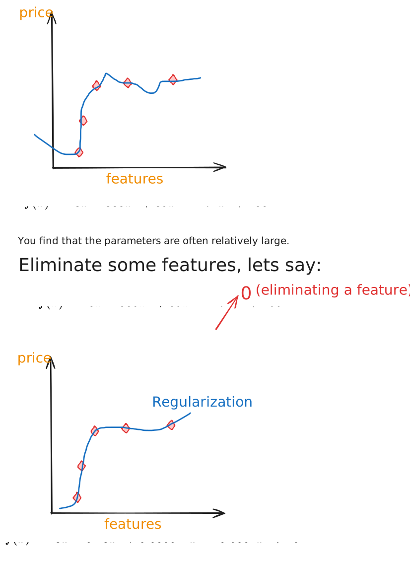
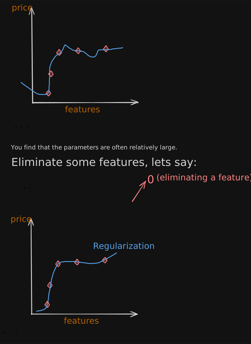
NOTE: setting a parameter to 0 is equivalent to eliminating a feature

It turns out that regularization is a way to more gently reduce the impacts of some of the features without doing something as harsh as eliminating them outright.
What regularization does is encourage the learning algorithm to shrink the values of the parameters without necessarily demanding that the parameter is set to exactly 0.
It turns out that even if you fit a higher order polynomial like this, so long as you can get the algorithm to use smaller parameter values: $w_1, w_2, w_3, w_4$ , you end up with a curve that ends up fitting the training data much better.
So what regularization does is let you keep all of your features, but it just prevents the features from having an overly large effect, which is what sometimes can cause overfitting.
By the way, by convention, we normally just reduce the size of the wj parameters, that is w1 through wn. It doesn’t make a huge difference whether you regularize the parameter b as well, you could do so if you want or not if you don’t. I usually don’t and it’s just fine to regularize w1, w2, all the way to wn, but not really encourage b to become smaller. In practice, it should make very little difference whether you also regularize b or not.

Recap¶

There are three ways to address overfitting:

Collect more data
Select Features (Feature Selection)
Reduce size of parameters using “Regularization”

Regularization¶

Reduce size of parameters

Cost Function with Regularization¶

We saw that regularization tries to make the parameter values $w_1$ through $w_n$ small to reduce overfitting. In this section, we’ll build on that intuition and develop a modified cost function for your learning algorithm that it can use to actually apply regularization.

Intuition¶

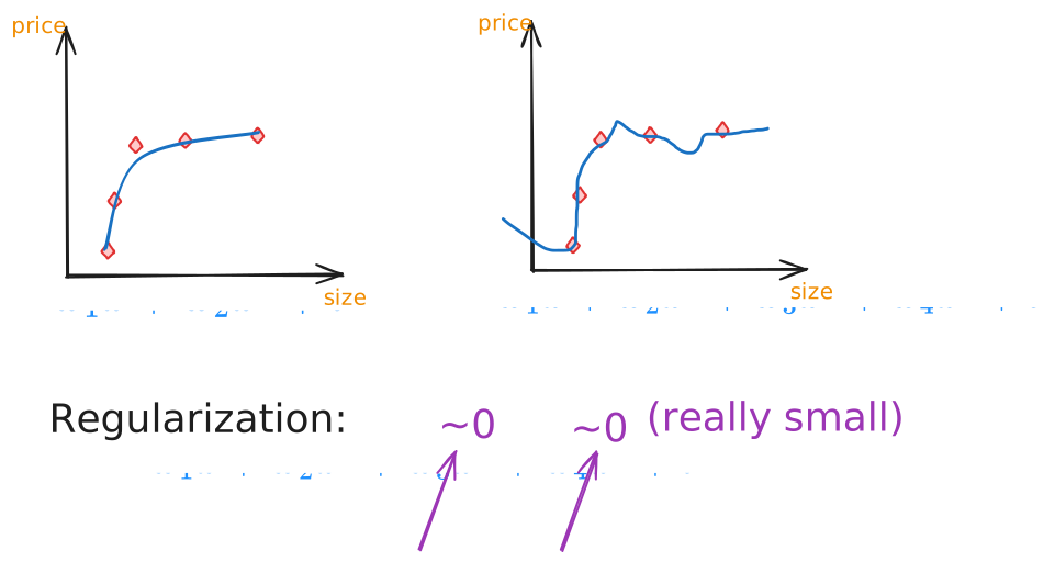
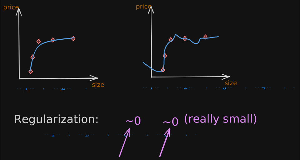
make $w_3, w_4$ really small ( $\approx 0$ )

Let’s say that instead of minimizing this cost function for linear regression,

you modify it and add to it 1000 times $w_3$ squared plus 1000 times $w_4$ squared.
- And here I’m just choosing 1000 because it’s a big number but any other really large number would be okay.
So with this modified cost function, you could in fact be penalizing the model if W3 and W4 are large.

\underset{\vec{w}, b}{\text{min}} \frac{1}{2m} \sum_{i = 1}^{m} (f_{\vec{w}, b} (\vec{X}^{(i)}) - y^{(i)})^2 + 1000w_{3}^2 + 1000 w_{4}^2

(6.1)

Because if you want to minimize this function, the only way to make this new cost function small is if $W_3$ and $W_4$ are both small, right?

Because otherwise this 1000 times W3 squared and 1000 times $W_4$ squared terms are going to be really, really big. So when you minimize this function, you’re going to end up with W3 close to 0 and $W_4$ close to 0.

So we’re effectively nearly canceling out the effects of the features x cubed and x to the power of 4 and getting rid of these two terms over here.

And if we do that, then we end up with a fit to the data that’s much closer to the quadratic function, including maybe just tiny contributions from the features x cubed and x to the fourth.

And this is good because it’s a much better fit to the data compared to if all the parameters could be large and you end up with this wiggly function.

Regularization¶

more generally, here’s the idea behind regularization.

The idea is that if there are smaller values for the parameters, then that’s a bit like having a simpler model. Maybe one with fewer features, which is therefore less prone to overfitting. On the last slide we penalized, or regularized only W3 and W4. But more generally, the way that regularization tends to be implemented is if you have a lot of features, say 100 features, you may not know which are the most important features and which ones to penalize.

So the way regularization is typically implemented is to penalize all of the features or more precisely, you penalize all the WJ parameters and it’s possible to show that this will usually result in fitting a smoother, simpler, less wiggly function that’s less prone to overfitting.

So for this example, if you have data with 100 features for each house, it may be hard to pick in advance which features to include and which ones to exclude.

So let’s build a model that uses all $n$ features.

J(\vec{w}, b) = \frac{1}{2m} \sum_{i = 1}^{m} (f_{\vec{w}, b} (\vec{X}^{(i)}) - y^{(i)}) ^ 2 + \frac{\lambda}{2m} \sum_{j = 1}^{n} w_{j}^2 + \frac{\lambda}{2m}b^2

(6.2)

$\lambda$ : This value lambda here is the Greek letter lambda and it’s also called a regularization parameter.
- So similar to picking a learning rate alpha, you now also have to choose a number for lambda.
- $\lambda > 0$
We also divide lambda by 2m so that both the 1st and 2nd terms here are scaled by 1 over 2m. It turns out that by scaling both terms the same way it becomes a little bit easier to choose a good value for lambda. And in particular you find that even if your training set size grows, say you find more training examples. the same value of λ is more likely to keep working even as m gets bigger.
by convention we’re not going to penalize the parameter b for being large.
- In practice, it makes very little difference whether you do or not.
- this makes very little difference in practice and the more common convention which was used in this book is to regularize only the parameters w rather than the parameter b.

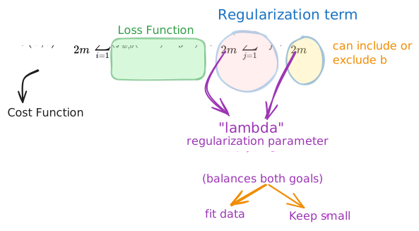
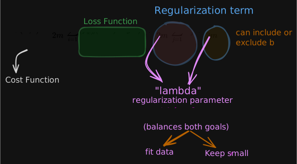
So to summarize in this modified cost function, we want to minimize the original cost, which is the mean squared error cost plus additionally, the second term which is called the regularization term. And so this new cost function trades off two goals that you might have.
Trying to minimize this first term encourages the algorithm to fit the training data well by minimizing the squared differences of the predictions and the actual values.
And by trying to minimize the second term, the algorithm also tries the second term. The algorithm also tries to keep the parameters wj small, which will tend to reduce overfitting.
The value of lambda that you choose specifies the relative importance or the relative trade-off or how you balance between these two goals.

Choosing Lambda¶

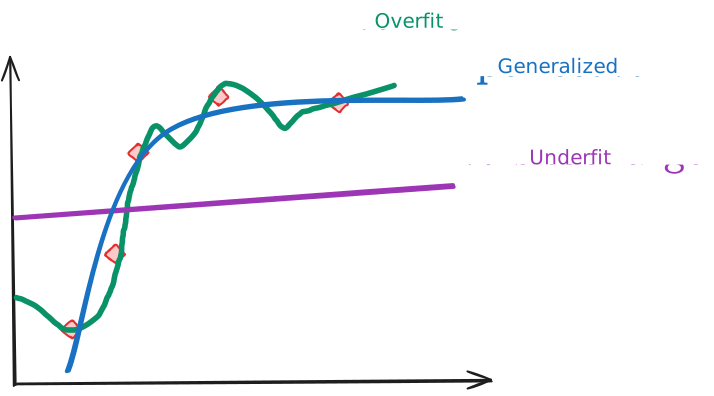
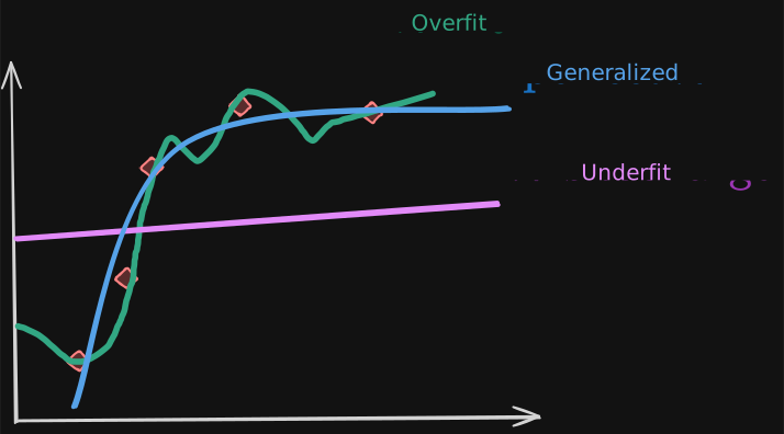
$\lambda = 0$ --> Overfits: If lambda were set to 0, then you’re not using the regularization term at all because the regularization term is multiplied by 0.
$\lambda$ really large --> Underfits: If you set lambda to be a really, really, really large number, say lambda equals 10 to the power of 10, then you’re placing a very heavy weight on this regularization term on the right. And the only way to minimize this is to be sure that all the values of w are pretty much very close to 0. So if lambda is very, very large, the learning algorithm will choose W1, W2, W3 and W4 to be extremely close to 0 and thus $f(X)$ is basically equal to b and so the learning algorithm fits a horizontal straight line and underfits.
Choose $\lambda$ in between that balances: some value of lambda that is in between that more appropriately balances these first and second terms of trading off, minimizing the mean squared error and keeping the parameters small.

Regularized Linear Regression¶

Here is a cost function for regularized linear regression:

J(\vec{w}, b) = \frac{1}{2m} \sum_{i = 1}^{m} (f_{\vec{w}, b} (\vec{X}^{(i)}) - y^{(i)})^2 + \frac{\lambda}{2m}\sum_{j = 1}^{n} w_{j}^2

(6.3)

our task is to

\underset{\vec{w}, b}{\text{min }} J(\vec{w}, b) = \underset{\vec{w}, b}{\text{min }} \frac{1}{2m} \sum_{i = 1}^{m} (f_{\vec{w}, b} (\vec{X}^{(i)}) - y^{(i)})^2 + \frac{\lambda}{2m}\sum_{j = 1}^{n} w_{j}^2

(6.4)

Gradient Descent is:

\begin{aligned} &repeat \ until \ convergence \ \{ \\ &w = w - \alpha \frac{d}{dw}J(w, b) \\ &b = b - \alpha \frac{d}{db}J(w, b) \\ &\} \text{ simultaneous update} \end{aligned}

(6.5)

Previously:

\frac{\partial}{\partial w_{j}} J(\vec{w}, b) = \frac{1}{m} \sum_{i=1}^{m} (f_{\vec{w}, b} (\vec{X}^{(i)}) - y^{(i)}) x_{j}^{(i)}

(6.6)

and

\frac{\partial}{\partial b} J(\vec{w}, b) = \frac{1}{m} \sum_{i=1}^{m} (f_{\vec{w}, b} (\vec{X}^{(i)}) - y^{(i)})

(6.7)

Now that we’ve added this additional regularization term, the only thing that changes is:

\frac{\partial}{\partial w_{j}} J(\vec{w}, b) = \frac{1}{m} \sum_{i=1}^{m} (f_{\vec{w}, b} (\vec{X}^{(i)}) - y^{(i)}) x_{j}^{(i)} + \frac{\lambda}{m}w_{j}

(6.8)

and we are not regularizing b, so it stays the same:

\frac{\partial}{\partial b} J(\vec{w}, b) = \frac{1}{m} \sum_{i=1}^{m} (f_{\vec{w}, b} (\vec{X}^{(i)}) - y^{(i)})

(6.9)

Let’s take these definitions for the derivatives and put them back into the expression on the left to write out the gradient descent algorithm for regularized linear regression.

\begin{aligned} &\text{repeat until convergence} \{ \\ & w_{j} = w_{j} - \alpha \big[ \frac{1}{m}\sum_{i=1}^{m} \big[(f_{w,b}(x^{(i)}) - y^{(i)}) x^{(i)}\big] + \frac{\lambda}{m}w_{j} \big] \\ &b = b - \alpha \frac{1}{m}\sum_{i=1}^{m} (f_{w,b}(x^{(i)}) - y^{(i)}) \\ & \} \text{ simultaneous update} \end{aligned}

(6.10)

Deeper Intuition (Math)¶

w_{j} = w_{j} - \alpha \big[ \frac{1}{m}\sum_{i=1}^{m} \big[(f_{w,b}(x^{(i)}) - y^{(i)}) x^{(i)}\big] + \frac{\lambda}{m}w_{j} \big]

(6.11)

Rewrite it as:

w_{j} = 1 w_{j} - \alpha \frac{\lambda}{m} w_{j} - \alpha \frac{1}{m} \sum_{i=1}^{m} (f_{\vec{w}, b} (\vec{X}^{(i)}) - y^{(i)}) X_{j}^{(i)}

(6.12)

Simplifying:

w_{j} = w_{j} \left( 1 - \alpha \frac{\lambda}{m} \right) - \alpha \frac{1}{m} \sum_{i=1}^{m} (f_{\vec{w}, b} (\vec{X}^{(i)}) - y^{(i)}) X_{j}^{(i)}

(6.13)

You might recognize the second term as the usual gradient descent update for unregularized linear regression. This is the update for linear regression before we had regularization.

Intuition: Let’s say $\lambda$ is 1 for this example and $m$ is the training set size, say 50. When you multiply $\alpha \frac{\lambda}{m}$ , say 0.01 times 1 divided by 50, this term ends up being a small positive number, say 0.0002, and thus, $1 - \alpha \frac{\lambda}{m}$ is going to be a number just slightly less than 1, in this case, 0.9998.

The effect of this term is that on every single iteration of gradient descent, you’re taking $w_j$ and multiplying it by 0.9998, that is by some number slightly less than one, before carrying out the usual update.
What regularization is doing on every single iteration is you’re multiplying w by a number slightly less than 1, and that has the effect of shrinking the value of w_j just a little bit. This gives us another view on why regularization has the effect of shrinking the parameters w_j a little bit on every iteration, and so that’s how regularization works.

How we get the derivative term¶

\frac{\partial}{\partial w_{j}} J(\vec{w}, b) = \frac{\partial}{\partial w_{j}} \big[\frac{1}{2m} \sum_{i=1}^{m} (f(\vec{X}^{(i)})- y^{(i)})^2 + \frac{\lambda}{2m} \sum_{j=1}^{n} w_{j}^2 \big]

(6.14)

= \frac{1}{2m} \sum_{i=1}^{m} \big[ (\vec{w}.\vec{X}^{(i)} + b - y^{(i)}) 2x_{j}^{(i)} \big] + \frac{\lambda}{2m} 2 w_{j}

(6.15)

= \frac{1}{m} \sum_{i=1}^{m} \big[ (\vec{w}.\vec{X}^{(i)} + b - y^{(i)}) x_{j}^{(i)} \big] + \frac{\lambda}{m} w_{j}

(6.16)

You now know how to implement regularized linear regression.

Using this, you can really reduce overfitting when you have a lot of features and a relatively small training set. This should let you get linear regression to work much better on many problems.

Regularized Logistic Regression¶

Cost Function for Logistic Regression:

J(\vec{w}, b) = -\frac{1}{m} \sum_{i = 1}^{m} \big[ y^{(i)} \log(f_{\vec{w}, b}(\vec{X}^{(i)})) + (1-y^{(i)}) \log (1 - f_{\vec{w}. b} (\vec{X}^{(i)})) \big]

(6.17)

To add regularization, we just need to add:

J(\vec{w}, b) = -\frac{1}{m} \sum_{i = 1}^{m} \big[ y^{(i)} \log(f_{\vec{w}, b}(\vec{X}^{(i)})) + (1-y^{(i)}) \log (1 - f_{\vec{w}. b} (\vec{X}^{(i)})) \big] + \frac{\lambda}{2m} \sum_{j=1}^{n} w_{j}^2

(6.18)

When you minimize this cost function as a function of w and b, it has the effect of penalizing parameters w_1, w_2 through w_n, and preventing them from being too large.

\underset{\vec{w}, b}{\text{min }} J(\vec{w}, b) = \underset{\vec{w}, b}{\text{min }} -\frac{1}{m} \sum_{i = 1}^{m} \big[ y^{(i)} \log(f_{\vec{w}, b}(\vec{X}^{(i)})) + (1-y^{(i)}) \log (1 - f_{\vec{w}. b} (\vec{X}^{(i)})) \big] + \frac{\lambda}{2m} \sum_{j=1}^{n} w_{j}^2

(6.19)

Let’s implement gradient descent with regularization:

\begin{aligned} &\text{repeat \{} \\ &w_{j} = w_{j} - \alpha \frac{\partial}{\partial w_{j}} J(\vec{w}, b) \\ &b = b - \alpha \frac{\partial}{\partial b} J(\vec{w}, b) \\ &\} \text{ Simultaneous Updates} \end{aligned}

(6.20)

\begin{aligned} &\text{repeat \{} \\ &w_{j} = w_{j} - \alpha \left[ \frac{1}{m} \sum_{i = 1}^{m} (f_{\vec{w}, b} (\vec{X}^{(i)}) - y^{(i)}) x_{j}^{(i)} \right] + \frac{\lambda}{m} w_{j}\\ &b = b - \alpha \left[ \frac{1}{m} \sum_{i = 1}^{m} (f_{\vec{w}, b} (\vec{X}^{(i)}) - y^{(i)}) \right] \\ &\} \text{ Simultaneous Updates} \end{aligned}

(6.21)

b is not regularized, so its update doesn’t change.

Summary¶

To fit the model well:

Collect more data
Feature Selection
Regularization